1.6. Alignment for a parallel-beam tomography system
Due to the parallelism of the penetrating X-rays, 2D projections can be divided into independent 1D projection rows. Collecting 1D projections at a specific row angularly forms a sinogram, which is used to reconstruct a 2D slice of an object (Fig. 1.6.1). To ensure the independence of 1D projections at each row, it is crucial to maintain the rotation axis parallel to the imaging plane and perpendicular to each image row. This requirement is known as tomography alignment. In a synchrotron-based tomography system, the high configurability in using different optics magnifications and/or sample-detector distances often causes the rotation axis being misaligned with the imaging plane. As the result, alignment adjustments are necessary for different tomography setups.
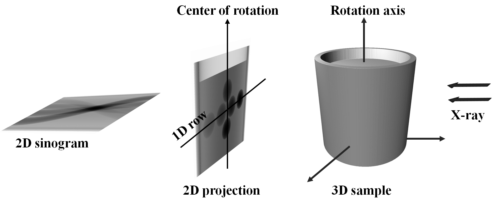
Fig. 1.6.1 Schematic of parallel-beam X-ray tomography.
The misalignment of a tomography system is identified by measuring the tilt and roll angle of the rotation axis relative to the imaging plane. This is achieved by scanning a point-like object, such as a sphere offset from the rotation axis, through a full rotation and tracking the trajectory of its center of mass, as illustrated in Fig. 1.6.2. A similar approach can be employed using a needle by tracking the top of it through a full rotation.
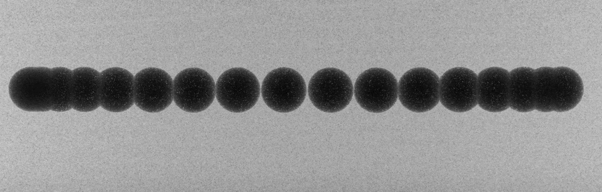
Fig. 1.6.2 Overlay of projections of a sphere during a circular scan.
In a well-aligned system, the range of y-coordinates of points remains below 1 pixel, as depicted in Fig. 1.6.3. If the system is misaligned, the y-coordinates of points will appear as an ellipse; where the roll angle corresponds to the angle of the major axis, and the tilt is related to the ratio between the minor and major axes of the ellipse.
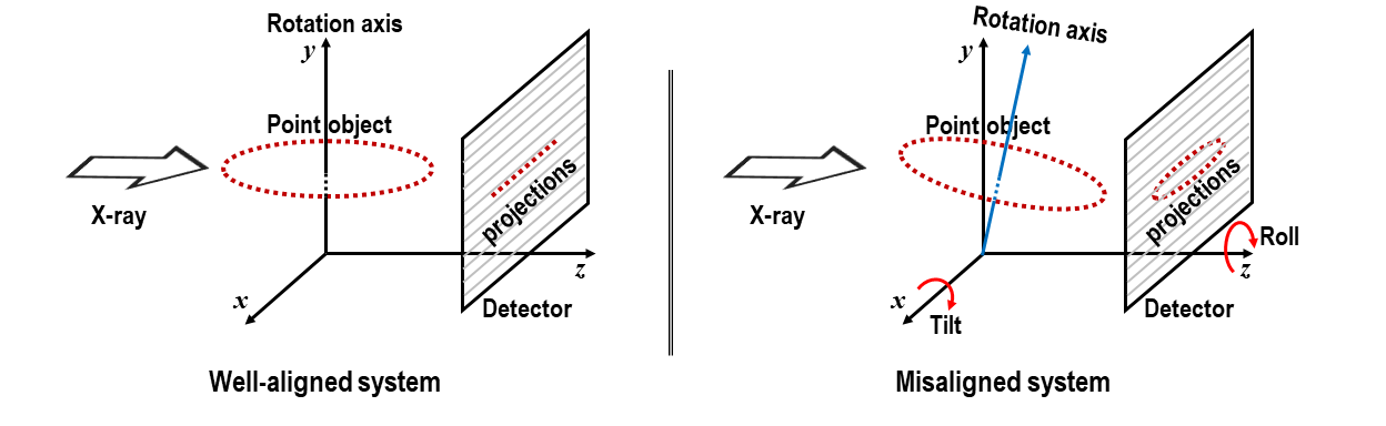
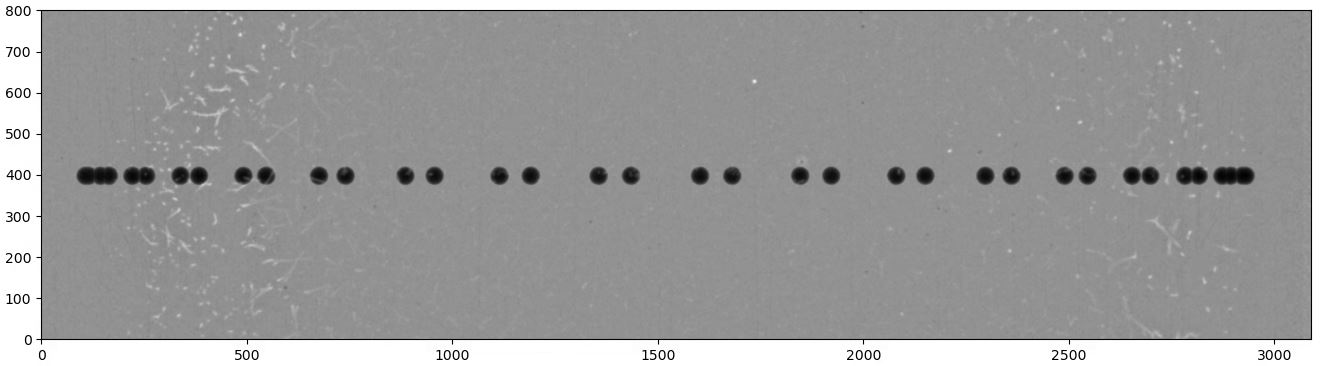
Fig. 1.6.3 Demonstration of a well-aligned tomography system and a misaligned one
This section demonstrates how to use methods available in Algotom to calculate the tilt and roll angle of the rotation axis from projections of a sphere scanned over the range of [0, 360] degrees.
Load the raw data and the corresponding flat-field images:
import numpy as np
import scipy.ndimage as ndi
import matplotlib.pyplot as plt
import algotom.io.loadersaver as losa
import algotom.util.calibration as calib

proj_path = "/tomo/data/scan_00001/"
flat_path = "/tomo/data/scan_00002/"

# If inputs are tif files
proj_files = losa.find_file(proj_path + "/*.tif*")
flat_files = losa.find_file(flat_path + "/*.tif*")
proj_data = np.asarray([losa.load_image(file) for file in proj_files])
flat = np.mean(np.asarray([losa.load_image(file) for file in flat_files]),
               axis=0)

# # If inputs are hdf files
# hdf_key = "entry/data/data"  # Change to the correct key.
# proj_data = losa.load_hdf(proj_path, hdf_key)
# (depth, height, width) = proj_data.shape
# flat = np.mean(np.asarray(losa.load_hdf(flat_path, hdf_key)), axis=0)
flat[flat == 0.0] = np.mean(flat)

have_flat = True
fit_ellipse = True  # Use an ellipse-fit method
ratio = 1.0  # To adjust the threshold for binarization

crop_left = 10
crop_right = 10
crop_top = 1000
crop_bottom = 1000

figsize = (15, 7)
(depth, height, width) = proj_data.shape
left = crop_left
right = width - crop_right
top = crop_top
bottom = height - crop_bottom
width_cr = right - left
height_cr = bottom - top
For each projection, multiple preprocessing steps are applied to segment the sphere and determine its center of mass. These steps include flat-field correction, background removal, binarization, and the removal of non-spherical objects, as follows:
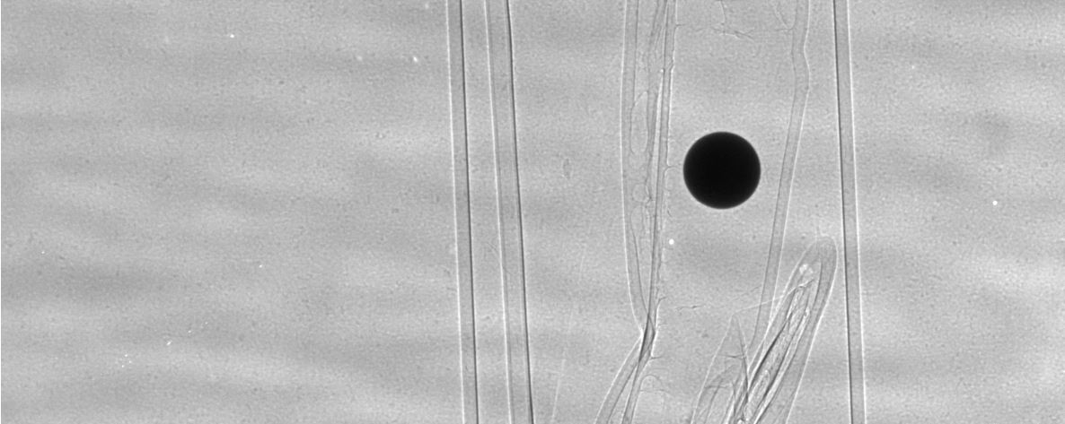
Fig. 1.6.4 Projection of the sphere
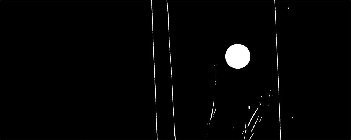
Fig. 1.6.5 Binarized image

Fig. 1.6.6 Segmented sphere
x_centers = []
y_centers = []
img_list = []
print("\n=============================================")
print("Extract the sphere and get its center-of-mass\n")

for i, img in enumerate(proj_data):
    # Crop image and perform flat-field correction
    if have_flat:
        mat = img[top: bottom, left:right] / flat[top: bottom, left:right]
    else:
        mat = img[top: bottom, left:right]
    # Denoise
    mat = ndi.gaussian_filter(mat, 2)
    # Normalize the background.
    # Optional, should be used if there's no flat-field.
    mat = calib.normalize_background_based_fft(mat, 5)
    threshold = calib.calculate_threshold(mat, bgr='bright')
    # Binarize the image
    mat_bin0 = calib.binarize_image(mat, threshold=ratio * threshold, bgr='bright')
    sphere_size = calib.get_dot_size(mat_bin0, size_opt="max")
    # Keep the sphere only
    mat_bin = calib.select_dot_based_size(mat_bin0, sphere_size)
    nmean = np.sum(mat_bin)
    if nmean == 0.0:
        print("\n************************************************************************")
        print("Adjust threshold or crop the FOV to remove objects larger than the sphere!")
        print("Current threshold used: {}".format(threshold))
        print("**************************************************************************")
        plt.figure(figsize=figsize)
        plt.imshow(mat_bin0, cmap="gray")
        plt.show()
        raise ValueError("No binary object selected!")
    (y_cen, x_cen) = ndi.center_of_mass(mat_bin)
    x_centers.append(x_cen)
    y_centers.append(height_cr - y_cen)
    img_list.append(mat)
    print("  ---> Done image: {}".format(i))
x = np.float32(x_centers)
y = np.float32(y_centers)
img_list = np.asarray(img_list)
img_overlay = np.min(img_list, axis=0)
The coordinates of the center of mass of the sphere are used to calculate the till and roll either using an ellipse-fit method or a linear-fit method.
# ==============================================================================

def fit_points_to_ellipse(x, y):
    if len(x) != len(y):
        raise ValueError("x and y must have the same length!!!")
    A = np.array([x ** 2, x * y, y ** 2, x, y, np.ones_like(x)]).T
    vh = np.linalg.svd(A, full_matrices=False)[-1]
    a0, b0, c0, d0, e0, f0 = vh.T[:, -1]
    denom = b0 ** 2 - 4 * a0 * c0
    msg = "Can't fit to an ellipse!!!"
    if denom == 0:
        raise ValueError(msg)
    xc = (2 * c0 * d0 - b0 * e0) / denom
    yc = (2 * a0 * e0 - b0 * d0) / denom
    roll_angle = np.rad2deg(
        np.arctan2(c0 - a0 - np.sqrt((a0 - c0) ** 2 + b0 ** 2), b0))
    if roll_angle > 90.0:
        roll_angle = - (180 - roll_angle)
    if roll_angle < -90.0:
        roll_angle = (180 + roll_angle)
    a_term = 2 * (a0 * e0 ** 2 + c0 * d0 ** 2 - b0 * d0 * e0 + denom * f0) * (
            a0 + c0 + np.sqrt((a0 - c0) ** 2 + b0 ** 2))
    if a_term < 0.0:
        raise ValueError(msg)
    a_major = -2 * np.sqrt(a_term) / denom
    b_term = 2 * (a0 * e0 ** 2 + c0 * d0 ** 2 - b0 * d0 * e0 + denom * f0) * (
            a0 + c0 - np.sqrt((a0 - c0) ** 2 + b0 ** 2))
    if b_term < 0.0:
        raise ValueError(msg)
    b_minor = -2 * np.sqrt(b_term) / denom
    if a_major < b_minor:
        a_major, b_minor = b_minor, a_major
        if roll_angle < 0.0:
            roll_angle = 90 + roll_angle
        else:
            roll_angle = -90 + roll_angle
    return roll_angle, a_major, b_minor, xc, yc

# ==============================================================================
# Calculate the tilt and roll using an ellipse-fit or a linear-fit method

if fit_ellipse is True:
    (a, b) = np.polyfit(x, y, 1)[:2]
    dist_list = np.abs(a * x - y + b) / np.sqrt(a ** 2 + 1)
    dist_list = ndi.gaussian_filter1d(dist_list, 2)
    if np.max(dist_list) < 1.0:
        fit_ellipse = False
        print("\nDistances of points to a fitted line is small, "
              "Use a linear-fit method instead!\n")

if fit_ellipse is True:
    try:
        result = fit_points_to_ellipse(x, y)
        roll_angle, major_axis, minor_axis, xc, yc = result
        tilt_angle = np.rad2deg(np.arctan2(minor_axis, major_axis))
    except ValueError:
        # If can't fit to an ellipse, using a linear-fit method instead
        fit_ellipse = False
        print("\nCan't fit points to an ellipse, using a linear-fit method instead!\n")

if fit_ellipse is False:
    (a, b) = np.polyfit(x, y, 1)[:2]
    dist_list = np.abs(a * x - y + b) / np.sqrt(a ** 2 + 1)
    appr_major = np.max(np.asarray([np.sqrt((x[i] - x[j]) ** 2 +
                                            (y[i] - y[j]) ** 2)
                                    for i in range(len(x))
                                    for j in range(i + 1, len(x))]))
    dist_list = ndi.gaussian_filter1d(dist_list, 2)
    appr_minor = 2.0 * np.max(dist_list)
    tilt_angle = np.rad2deg(np.arctan2(appr_minor, appr_major))
    roll_angle = np.rad2deg(np.arctan(a))

print("=============================================")
print("Roll angle: {} degree".format(roll_angle))
print("Tilt angle: {} degree".format(tilt_angle))
print("=============================================\n")
Show the results:
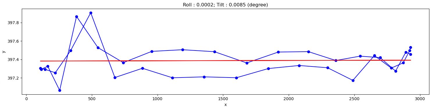
# Show the results
plt.figure(1, figsize=figsize)
plt.imshow(img_overlay, cmap="gray", extent=(0, width_cr, 0, height_cr))
plt.tight_layout(rect=[0, 0, 1, 1])

plt.figure(0, figsize=figsize)
plt.plot(x, y, marker="o", color="blue")
plt.title(
    "Roll : {0:2.4f}; Tilt : {1:2.4f} (degree)".format(roll_angle, tilt_angle))
if fit_ellipse is True:
    # Use parametric form for plotting the ellipse
    angle = np.radians(roll_angle)
    theta = np.linspace(0, 2 * np.pi, 100)
    x_fit = (xc + 0.5 * major_axis * np.cos(theta) * np.cos(
        angle) - 0.5 * minor_axis * np.sin(theta) * np.sin(angle))
    y_fit = (yc + 0.5 * major_axis * np.cos(theta) * np.sin(
        angle) + 0.5 * minor_axis * np.sin(theta) * np.cos(angle))
    plt.plot(x_fit, y_fit, color="red")
else:
    plt.plot(x, a * x + b, color="red")
plt.xlabel("x")
plt.ylabel("y")
plt.tight_layout()
plt.show()
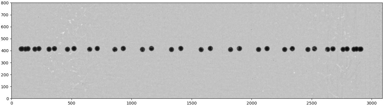
Fig. 1.6.7 Overlay of projections of a sphere for checking.
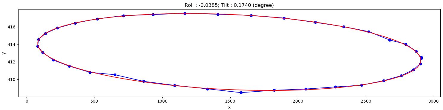
Fig. 1.6.8 Showing the result of finding the tilt and roll.
From the given results, we can adjust the rotation axis or the detector system accordingly. Note that the calculated angles are based only on input images, so the sign of the angles does not reflect the true geometry of a tomography system. Using information such as the direction of rotation when scanning spheres and/or camera orientation, we can correctly identify the sign of these angles. After the adjustment, calculation results should be as follows:
The above routine performs very well in practice. However, if the projection images are of low quality due to blobs on the scintillator or optics system, an additional cleaning step for image processing (using some functions in the scikit-image library) can be included as follows:
from skimage import measure, segmentation

def remove_non_round_objects(binary_image, ratio_threshold=0.9):
    """
    To clean binary image and remove non-round objects
    """
    binary_image = segmentation.clear_border(binary_image)
    binary_image = ndi.binary_fill_holes(binary_image)
    label_image = measure.label(binary_image)
    properties = measure.regionprops(label_image)
    mask = np.zeros_like(binary_image, dtype=bool)
    # Filter objects based on the axis ratio
    for prop in properties:
        if prop.major_axis_length > 0:
            axis_ratio = prop.minor_axis_length / prop.major_axis_length
            if axis_ratio > ratio_threshold:
                mask[label_image == prop.label] = True
    # Apply mask to keep only round objects
    filtered_image = np.logical_and(binary_image, mask)
    return filtered_image

# ...
# Binarize the image
mat_bin0 = calib.binarize_image(mat, threshold=ratio * threshold, bgr='bright')
# Clean the image
mat_bin0 = remove_non_round_objects(mat_bin0)
sphere_size = calib.get_dot_size(mat_bin0, size_opt="max")
# Keep the sphere only
# ...
The complete script and its commandline user interface (CLI) version are available here. If users prefer an interactive way of assessing tomographic alignment as shown below, the ImageJ macros can be downloaded from here.
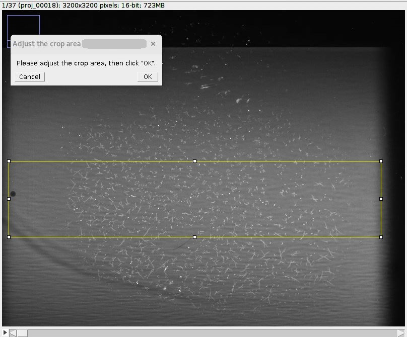
Fig. 1.6.11 Interactive approach for tomography alignment using ImageJ macro.