4.2. Exploring raw data and making use of the input-output module

The following sections show how to handle different types of raw data before they can be used for processing and reconstruction.

4.2.1. Nxs/hdf files

A nxs/hdf file can contain multiple datasets and data-types. Generally speaking, it likes a folder with many sub-folders and files inside (i.e. hierarchical format). To get data from a hdf file we need to know the path to the data. For example, we want to know the path to projection-images of this tomographic data. The data have two files: a hdf file which contains images recorded by a detector and a nxs file which contains the metadata of the experiment. The hdf file was linked to the nxs file at the time they were created, so we only need to work with the nxs file.

Using Hdfview (version 2.14 is easy to install) we can find the path to image data is “/entry1/tomo_entry/data/data”. To display an image in that dataset: right click on “data” -> select “Open as” -> select “dim1” for “Height”, select “dim2” for “Width” -> click “OK”.

A metadata we need to know is rotation angles corresponding to the acquired images. The path to this data is “/entry1/tomo_entry/data/rotation_angle”. There are three types of images in a tomographic dataset: images with sample (projection), images without sample (flat-field or white field), and images taken with a photon source off (dark-field). In the data used for this demonstration, there’s a metadata in “/entry1/instrument/image_key/image_key” used to indicate the type of an image: 0 <-> projection; 1 <-> flat-field; 2 <-> dark-field.

Different tomography facilities name above datasets differently. Some names rotation angles as “theta_angle”. Some record flat-field and dark-field images as separate datasets (Fig. 1.4.1). There has been an effort to unify these terms for synchrotron-based tomography community. This will be very userful for end-users where they can use the same codes for processing data acquired at different facilities.
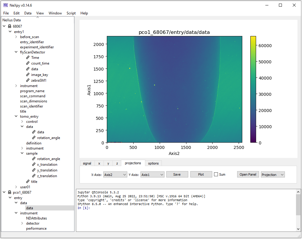
Other way of exploring nxs/hdf files is to use NeXpy. Users need to install NeXpy in an activated environment.
conda install -c conda-forge nexpy
and run from that environment

NeXpy provides more options to explore data. Noting that image in NeXpy is displayed with the origin at the bottom left. This is different to Hdfview (Fig. 1.4.2).

Other python-based GUI software can be used are: Broh5 or Vitables.

Users also can use functions in the input-output module of Algotom to explore data. For example, to display the hierarchical structure of a hdf file:

import algotom.io.loadersaver as losa

file_path = "E:/Tomo_data/68067.nxs"
losa.get_hdf_tree(file_path)

Output:
entry1
    │
    ├── before_scan
    │   │
    │   ├── cam1
    │   │   │
    │   │   ├── cam1_roll (1,)
    │   │   ├── cam1_x (1,)
    │   │   └── cam1_z (1,)
    │   ├── dcm1_cap_1
    │   │   └── dcm1_cap_1 (1,)

To find datasets having the pattern of “data” in their paths:

keys, shapes, types = losa.find_hdf_key(file_path, "data")
for i in range(len(keys)):
    print(i," Key: {0} | Shape: {1} | Type: {2} ".format(keys[i], shapes[i], types[i]))

Output:
Key: entry1/flyScanDetector/data | Shape: (1861, 2160, 2560) | Type: uint16
Key: entry1/instrument/flyScanDetector/data | Shape: (1861, 2160, 2560) | Type: uint16
Key: entry1/tomo_entry/data | Shape: None | Type: None
Key: entry1/tomo_entry/control/data | Shape: (1,) | Type: float64
Key: entry1/tomo_entry/data/data | Shape: (1861, 2160, 2560) | Type: uint16
Key: entry1/tomo_entry/data/rotation_angle | Shape: (1861,) | Type: float64
Key: entry1/tomo_entry/instrument/detector/data | Shape: (1861, 2160, 2560) | Type: uint16

After knowing the path (key) to a dataset containing images we can extract an image and save it as tif. A convenient feature of methods for saving data in Algotom is that if the output folder doesn’t exist it will be created.

image_data = losa.load_hdf(file_path, "entry1/tomo_entry/data/data")
losa.save_image("E:/output/image_00100.tif", image_data[100])

We also can extract multiple images from a hdf file and save them to tiff using a single command

import algotom.io.converter as conv

# Extract images with the indices of (start, stop, step) along axis 0
conv.extract_tif_from_hdf(file_path, "E:/output/some_proj/", "entry1/tomo_entry/data/data",
                          index=(0, -1, 100), axis=0, crop=(0, 0, 0, 0), prefix='proj')

4.2.2. Tiff files

In some tomography systems, raw data are saved as tiff images. As shown in section 2, processing methods for tomographic data work either on projection space or sinogram space, or on both. Because of that, we have to switch between spaces, i.e. slicing 3D data along different axis. This cannot be done efficiently if using the tiff format. In such case, users can convert tiff images to the hdf format first before processing them with options to add metadata.

input_folder = "E:/raw_tif/" # Folder with tiff files inside. Note that the names of the
                             # tiff files must be corresponding to the increasing order of angles
output_file = "E:/convert_hdf/tomo_data.hdf"
num_angle = len(losa.file_file(input_folder + "/*tif*"))
angles = np.linspace(0.0, 180.0, num_angle)
conv.convert_tif_to_hdf(input_folder, output_file, key_path='entry/data',
                        crop=(0, 0, 0, 0), pattern=None,
                        options={"entry/angles": angles, "entry/energy_keV": 20})

In some cases, we may want to load a stack of tiff images and average them such as flat-field images or dark-field images. This can be done in different ways

input_folder = "E:/flat_field/"
# 1st way
flat_field = np.mean(losa.get_tif_stack(input_folder, idx=None, crop=(0, 0, 0, 0)), axis=0)
# 2nd way. The method was written for speckle-tracking tomography but can be used here
flat_field = losa.get_image_stack(None, input_folder, average=True, crop=(0, 0, 0, 0))
# 3rd way
list_file = losa.find_file(input_folder + "/*tif*")
flat_field = np.mean(np.asarray([losa.load_image(file) for file in list_file]), axis=0)

4.2.3. Mrc files

Mrc format is a standard format in electron tomography. To load this data, users need to install the Mrcfile library

conda install -c conda-forge mrcfile

and check the documentation page to know how to extract data and metadata from this format. For large files, we use memory-mapped mode to read only part of data needed as shown below.

import mrcfile
import algotom.io.loadersaver as losa

mrc = mrcfile.mmap("E:/etomo/tomo.mrc", mode='r+')
output_base = "E:/output"
(depth, height, width) = mrc.data.shape
for i in range(0, depth, 10):
    name = "0000" + str(i)
    losa.save_image(output_base + "/img_" + name[-5:] + ".tif", mrc.data[i])

Methods in Algotom assume that the rotation axis of a tomographic data is parallel to the columns of an image. Users may need to rotate images loaded from a mrc file because the rotation axis is often parallel to image-rows instead.

4.2.4. Other file formats

For other file formats such as xrm, txrm, fits, … users can use the DXchange library to load data

conda install -c conda-forge dxchange

and refer the documentation page for more details.