4.5. Complete workflow for processing tomographic data
This guide presents a comprehensive workflow for processing tomographic data, starting from raw data. In addition, it includes useful tips and explanations to users’ common mistakes.
4.5.1. Assessing raw data
A typical tomographic dataset includes:
Raw data acquired by a detector which are: projection images, flat-field image, and dark-field images.
Metadata that provides information about the experimental setup, such as rotation angles, energy, pixel size, sample-detector distance, and any other relevant parameters.
Visual inspection (using ImageJ) can help determine whether raw data are of sufficient quality. Users may want to perform the following checks:
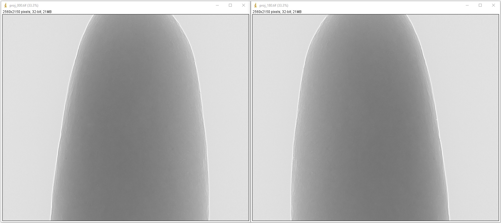
Verify that the first and the last projection are 180-degree apart:
If raw data are in hdf/h5/nxs format, the projections can be extracted and saved as tif images as the following:
import numpy as np
import algotom.io.loadersaver as losa

file_path = "E:/Tomo_data/scan_68067.hdf"
output_base = "E:/tmp/extract_tifs/"
proj_path = "entry/projections"  # Refer section 1.2.1 to know how to get
                                 # path to a dataset in a hdf file.
flat_path = "entry/flats"
flat_img = np.mean(np.asarray(losa.load_hdf(file_path, flat_path)), axis=0)
nmean = np.mean(flat_img)
flat_img[flat_img == 0.0] = nmean  # To avoid zero division

proj_obj = losa.load_hdf(file_path, proj_path)  # hdf object
proj_0 = proj_obj[0, :, :] / flat_img
losa.save_image(output_base + "/proj_0.tif", proj_0)
proj_180 = proj_obj[-1, :, :] / flat_img
losa.save_image(output_base + "/proj_180.tif", proj_180)
If the first and last projection are 180-degree apart, the second image should be a mirror reflection (left-right flip) of the first image.
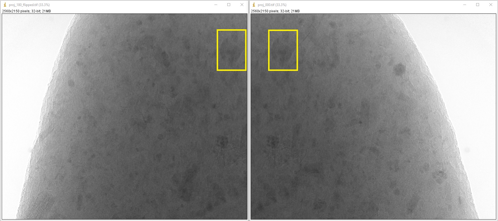
If data were acquired using a 360-degree scan with an offset rotation axis, it is important to verify that the rotation axis is positioned to one side of the field of view (FOV). This can be done by checking for an overlap between the 0-degree projection and the left-right flipped 180-degree projection image.
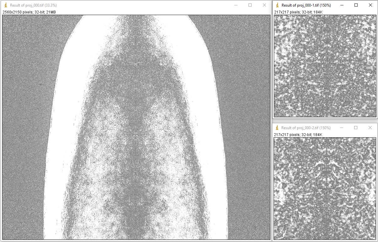
Check if the rotation axis is tilted. This can be done by calculating the difference/average between the 0-degree projection and the 180-degree projection, then examining the resulting image for a symmetric line. If the x-location of the symmetric line is the same at the top and bottom of the image, the rotation axis is properly aligned.
If a tilt is detected, the tilt angle can be accurately calculated by locating the center of rotation using sinograms generated at the top, middle, and bottom of the FOV; then applying a linear fit to the results. The resulting tilt angle can be used to correct the tilted tomographic images, as shown here.
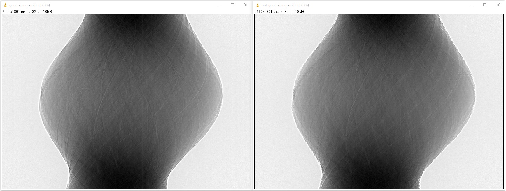
Ensure that projection images were acquired at evenly spaced angles and there was no stage jittering during the scan by inspecting a sinogram image:
If raw data are in hdf/h5/nxs format, the sinogram can be extracted and saved as tif format as follows:
import numpy as np
import algotom.io.loadersaver as losa

file_path = "E:/Tomo_data/scan_68067.hdf"
output_base = "E:/tmp/extract_tifs/"
proj_path = "entry/projections"  # Refer section 1.2.1 to know how to get
                                 # path to a dataset in a hdf file.
flat_path = "entry/flats"
flat_img = np.mean(np.asarray(losa.load_hdf(file_path, flat_path)), axis=0)
nmean = np.mean(flat_img)
flat_img[flat_img == 0.0] = nmean  # To avoid zero division

proj_obj = losa.load_hdf(file_path, proj_path)  # hdf object
(depth, height, width) = proj_obj.shape
sino_idx = height // 2
sinogram = proj_obj[:, sino_idx, :] / flat_img[sino_idx]
losa.save_image(output_base + "/sinogram.tif", sinogram)
If input data are in tif format, we need to convert them to the hdf format for fast extracting sinogram image:
import os
import shutil
import numpy as np
import algotom.io.converter as cvr
import algotom.io.loadersaver as losa

proj_path = "E:/Tomo_data/scan_68067/projections/"
flat_path = "E:/Tomo_data/scan_68067/flats/"

output_base = "E:/tmp/extract_tifs/"

flat_img = np.mean(np.asarray(
    [losa.load_image(file) for file in losa.find_file(flat_path + "/*tif*")]), axis=0)
nmean = np.mean(flat_img)
flat_img[flat_img == 0.0] = nmean  # To avoid zero division

# Convert data to hdf format for fast extracting sinograms.
hdf_file_path = output_base + "/hdf_converted/" + "tomo_data.hdf"
key_path = "entry/data"
cvr.convert_tif_to_hdf(proj_path, hdf_file_path, key_path=key_path)
proj_obj, hdf_obj = losa.load_hdf(hdf_file_path, key_path, return_file_obj=True)
(depth, height, width) = proj_obj.shape

sino_idx = height // 2
sinogram = proj_obj[:, sino_idx, :] / flat_img[sino_idx]
losa.save_image(output_base + "/sinogram.tif", sinogram)
hdf_obj.close()
# Remove the hdf file if needs to
if os.path.isdir(output_base + "/hdf_converted/"):
    shutil.rmtree(output_base + "/hdf_converted/")
4.5.2. Reconstructing several slices
In high throughput tomographic systems, it’s common that users want to quickly reconstruct only a few slices in order to verify the quality of the data or to locate the region of interest for higher resolution scans. This can be achieved by following these steps:
Load the raw data and the corresponding flat-field and dark-field images. It’s common to acquire multiple flat and dark images (usually between 10 and 50) and average them to improve the signal-to-noise (SNR) ratio. Once the flat and dark images have been averaged, they can be used for flat-field correction.
If raw data are in tif format, we need to convert them to hdf format first:
import numpy as np
import algotom.io.loadersaver as losa
import algotom.io.converter as cvr
import algotom.prep.correction as corr
import algotom.prep.calculation as calc
import algotom.prep.removal as remo
import algotom.prep.filtering as filt
import algotom.rec.reconstruction as rec


proj_path = "E:/Tomo_data/scan_68067_tif/projections/"
flat_path = "E:/Tomo_data/scan_68067_tif/flats/"
dark_path = "E:/Tomo_data/scan_68067_tif/darks/"

output_base = "E:/output/rec_few_slices/"

# Load dark-field images and flat-field images.
flats = losa.get_tif_stack(flat_path)
darks = losa.get_tif_stack(dark_path)

# Convert tif images to hdf format for fast extracting sinograms.
file_path = output_base + "/tmp_/" + "tomo_data.hdf"
key_path = "entry/projections"
cvr.convert_tif_to_hdf(proj_path, file_path, key_path=key_path,
                       option={"entry/flats": flats, "entry/darks": darks})
Working with a hdf file is straightforward as follows:
import numpy as np
import algotom.io.loadersaver as losa
import algotom.io.converter as cvr
import algotom.prep.correction as corr
import algotom.prep.calculation as calc
import algotom.prep.removal as remo
import algotom.prep.filtering as filt
import algotom.rec.reconstruction as rec


file_path = "E:/Tomo_data/scan_68067.hdf"
output_base = "E:/output/rec_few_slices/"
proj_path = "entry/projections"  # Refer section 1.2.1 to know how to get
                                 # path to a dataset in a hdf file.
flat_path = "entry/flats"
dark_path = "entry/darks"

# Load data, average flat and dark images
proj_obj = losa.load_hdf(file_path, proj_path)  # hdf object
(depth, height, width) = proj_obj.shape
flat_field = np.mean(np.asarray(losa.load_hdf(file_path, flat_path)), axis=0)
dark_field = np.mean(np.asarray(losa.load_hdf(file_path, dark_path)), axis=0)

# If the rotation angles are not provided, e.g. from metadata of the HDF file,
# they can be generated automatically in a reconstruction method. Note that
# the rotation angles are in radians as requested by the reconstruction method.
# To rotate the reconstructed image, simply add an offset angle using the following method:
offset_angle = 0.0  # Degree
angles = np.deg2rad(offset_angle + np.linspace(0.0, 180.0, depth))

# Specify the range of slices to be reconstructed
start_slice = 100
stop_slice = height - 100
step_slice = 100

# Extract sinogram at the middle for calculating the center of rotation
idx = height // 2
sinogram = corr.flat_field_correction(proj_obj[:, idx, :], flat_field[idx],
                                      dark_field[idx])
center = calc.find_center_vo(sinogram)
print("Center of rotation: {}".format(center))

# Extract sinograms and perform flat-field correction
for idx in range(start_slice, stop_slice + 1, step_slice):
    sinogram = corr.flat_field_correction(proj_obj[:, idx, :], flat_field[idx],
                                          dark_field[idx])
    # Apply pre-processing methods
Apply pre-processing methods: zinger removal, ring artifact removal, and/or denoising to sinograms. Note that there are many choices for ring-removal methods, but for this step we may just want a fast method.
# ...
    # Apply pre-processing methods
    sinogram = remo.remove_zinger(sinogram, 0.08)
    sinogram = remo.remove_stripe_based_normalization(sinogram, 15)
    sinogram = filt.fresnel_filter(sinogram, 100)
    # Perform reconstruction
Perform reconstruction and save the results to tif. Algotom provides reconstruction methods that can run on either CPU or GPU. It also provides the wrappers of the gridrec method, available in Tomopy, which is very fast for CPU-only computers; and iterative methods available in Astra Toolbox. Note that if users want to use these additional wrappers, Tomopy and Astra will need to be installed along with Algotom.
# ...
    # Perform reconstruction
    # Using a cpu method
    rec_img = rec.fbp_reconstruction(sinogram, center, angles=angles,
                                     apply_log=True, gpu=False)
    # # Other options:
    # rec_img = rec.dfi_reconstruction(sinogram, center, angles=angles,
    #                                  apply_log=True)
    # # Using a gpu method
    # rec_img = rec.fbp_reconstruction(sinogram, center, angles=angles,
    #                                  apply_log=True, gpu=True)
    # # Using a cpu method, available in Tomopy
    # rec_img = rec.gridrec_reconstruction(sinogram, center, angles=angles,
    #                                  apply_log=True)
    # # Using a gpu method, available in Astra Toolbox
    # rec_img = rec.astra_reconstruction(sinogram, center, angles=angles,
    #                                    method="SIRT_CUDA", num_iter=150,
    #                                    apply_log=True)
    out_file = output_base + "/rec_" + ("00000" + str(idx))[-5:] + ".tif"
    losa.save_image(out_file, rec_img)
4.5.3. Finding the center of rotation
Algotom offers several methods for automatically calculating the center of rotation (COR), which refers to the rotation axis of the sample stage with respect to the FOV. These methods work on different processing spaces (Fig. 4.5.1) and can be selected according to specific types of input images.
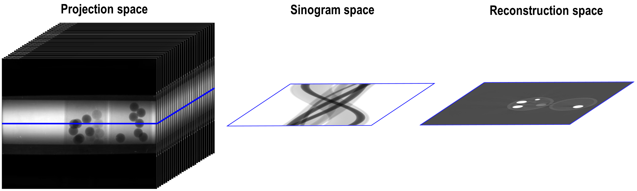
Fig. 4.5.1 Different processing spaces can be used for finding the center of rotation.
Methods that work in the projection space are the fastest and simplest, but they are also the least reliable.
import timeit
import algotom.prep.calculation as calc

# Data is at: https://doi.org/10.5281/zenodo.1443567
# Steps for loading data are similar to above sections

proj_0 = proj_obj[0, :, :] / flat_field
proj_180 = proj_obj[-1, :, :] / flat_field

print("Image size: {}".format(flat_field.shape))
t0 = timeit.default_timer()
center = calc.find_center_based_phase_correlation(proj_0, proj_180)
t1 = timeit.default_timer()
print("Using phase correlation. Center: {0}. Time: {1}".format(center, t1 -t0))

t0 = timeit.default_timer()
center = calc.find_center_projection(proj_0, proj_180, chunk_height=100)
t1 = timeit.default_timer()
print("Using image correlation. Center: {0}. Time: {1}".format(center, t1 -t0))
>>>
Image size: (2160, 2560)
Using phase correlation. Center: 1272.8564415436447. Time: 1.6949839999999998
Using image correlation. Center: 1272.8176879882812. Time: 15.652110699999998
The most reliable method for automatically calculating the center of rotation is a method that works on a 180-degree sinogram image, as proposed in [R21]. This method has been extensively tested on 2,000 micro-tomography datasets, achieving a success rate of 98%. A visual explanation of how the method works is provided in Fig. 4.5.2.
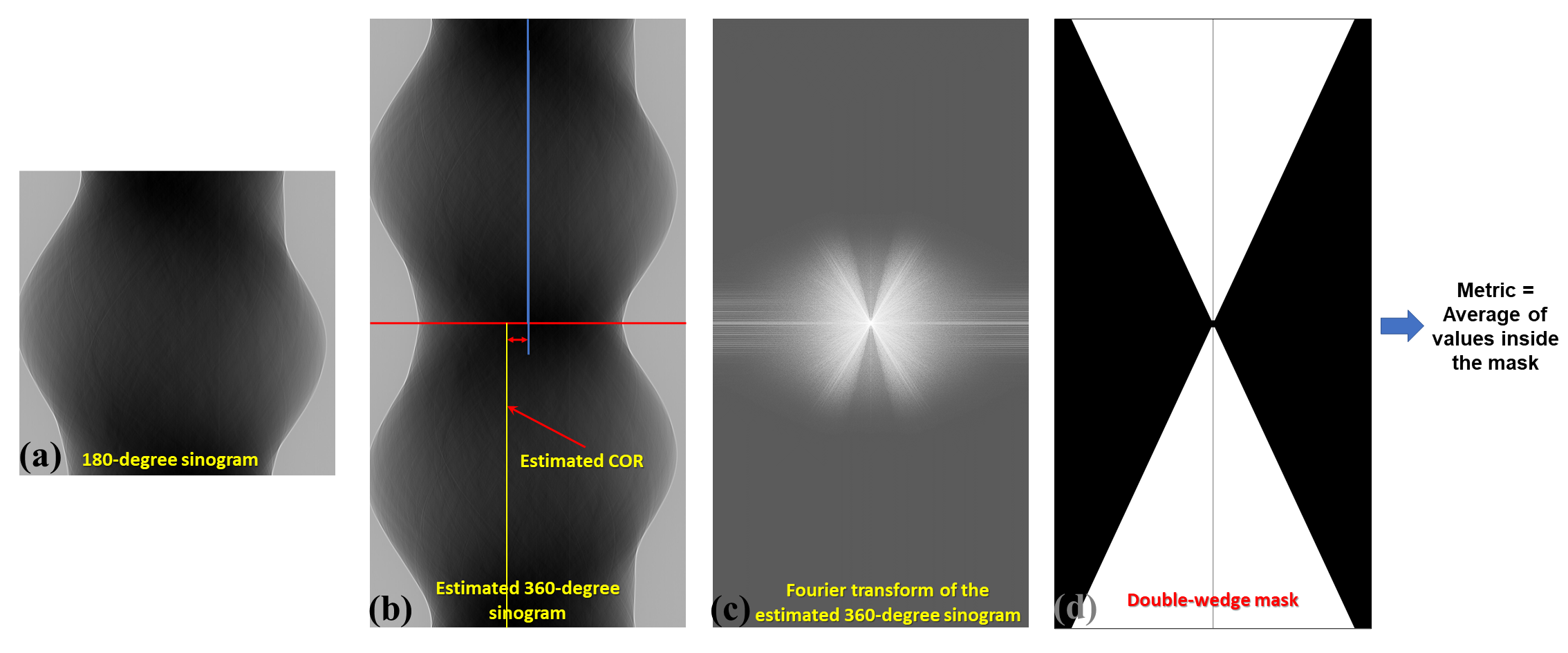
Fig. 4.5.2 Explanation of how the autocentering method in the sinogram space works.
idx = height // 2
sinogram = corr.flat_field_correction(proj_obj[:, idx, :], flat_field[idx],
                                      dark_field[idx])
t0 = timeit.default_timer()
radius = width // 16
mid = width // 2
# Enable parallel computing using the "ncore" option.
center = calc.find_center_vo(sinogram, start=mid - radius, stop=mid + radius,
                             ncore=8)
t1 = timeit.default_timer()
print("Using sinogram metric. Center: {0}. Time: {1}".format(center, t1 - t0))
>>>
Using sinogram metric. Center: 1272.75. Time: 8.0966264
The method’s default parameters work for most X-ray microtomography datasets, as extensively tested. However, users can adjust these parameters, such as the ratio and ver_drop parameters, to suit their data. A unique feature of this method is the ability to average multiple sinograms to improve the signal-to-noise ratio and use the result as input for the method. Note that strongly smoothed or blurry sinograms resulting from denoising methods or phase-retrieval methods can impact the performance of this method.
Another method, available from Algotom 1.3, works in the reconstruction space and evaluates a slice metric to determine the best center of rotation. This method is slower than the other methods and is most suitable for performing small, fine searching ranges around the coarse center found by previous methods. It may not be suitable for use on low SNR data.
import algotom.rec.reconstruction as rec

t0 = timeit.default_timer()
center = rec.find_center_based_slice_metric(sinogram, mid-radius, mid + radius,
                                            zoom=0.5, method='fbp', gpu=True,
                                            apply_log=True)
t1 = timeit.default_timer()
print("Using slice metric. Reconstruction method: FBP. Center: {0}. Time: {1}".format(center, t1 - t0))

t0 = timeit.default_timer()
center = rec.find_center_based_slice_metric(sinogram, mid-radius, mid + radius,
                                            zoom=0.5, method='dfi',
                                            apply_log=True)
t1 = timeit.default_timer()
print("Using slice metric. Reconstruction method: DFI. Center: {0}. Time: {1}".format(center, t1 - t0))

t0 = timeit.default_timer()
center = rec.find_center_based_slice_metric(sinogram, mid-radius, mid + radius,
                                            zoom=0.5, method='gridrec',
                                            apply_log=True)
t1 = timeit.default_timer()
print("Using slice metric. Reconstruction method: Gridrec. Center: {0}. Time: {1}".format(center, t1 - t0))
>>>
Using slice metric. Reconstruction method: FBP. Center: 1272.5. Time: 104.3659703
Using slice metric. Reconstruction method: DFI. Center: 1272.5. Time: 85.9248028
Using slice metric. Reconstruction method: Gridrec. Center: 1272.5. Time: 14.54944309999999
If users would like to apply a customized function for calculating a slice metric, it can be done as follows:
def measure_metric(mat, n=2):
    metric = np.abs(np.mean(mat[mat < 0.0])) ** n
    return metric
center = rec.find_center_based_slice_metric(sinogram, mid-10, mid + 10,
                                            zoom=1.0, method='fbp', gpu=True,
                                            apply_log=True,
                                            metric_function=measure_metric, n=2)
If the automated methods fail to find the center of rotation, users can rely on the following manual methods (available from Algotom 1.3) to locate it:
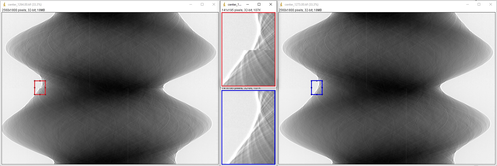
The first manual method involves generating a list of 360-degree sinograms created from the input 180-degree sinogram using a list of estimated CORs. Users can find the best COR by identifying the generated sinogram that has a continuous transition between the two halves of the sinogram, as illustrated in the figure below.
import algotom.util.utility as util

output_base = "E:/tmp/manual_finding/using_sinograms/"
util.find_center_visual_sinograms(sinogram, output_base, width // 2 - 20, width // 2 + 20,
                                  step=1, zoom=1.0)
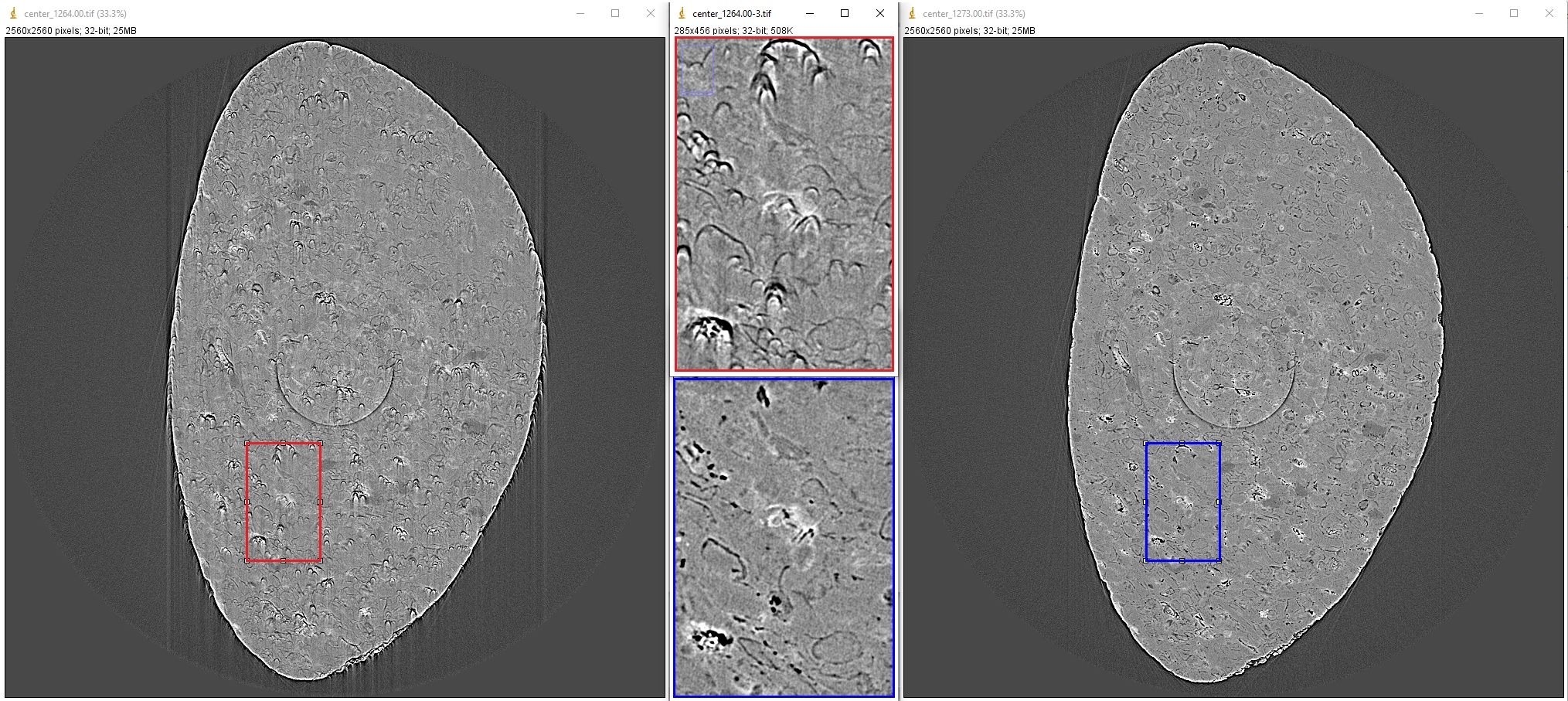
The second manual method involves reconstructing a list of slices using a list of estimated CORs. Users can find the best COR by visually inspecting the reconstructed slices and selecting the one with the least streak artifacts.
import algotom.rec.reconstruction as rec

output_base = "E:/tmp/manual_finding/using_slices/"
rec.find_center_visual_slices(sinogram, output_base, width // 2 - 20,
                              width // 2 + 20, 1, zoom=1.0, method="fbp", gpu=True)
4.5.4. Tweaking parameters of preprocessing methods
When reconstructing synchrotron-based X-ray microtomography data, users often spend most of time tweaking parameters of preprocessing methods such as ring artifact removal or contrast-enhancement methods. We can setup different workflows to test methods as below:
To compare different ring removal methods; note that in Algotom, some well-known methods are improved and have additional options for customization:
# Steps for loading data are similar to above sections

# To create new output-folder for each time of running the script.
output_base0 = "E:/tmp/compare_ring_removal_methods/"
folder_name = losa.make_folder_name(output_base0, name_prefix="Ring_removal", zero_prefix=3)
output_base = output_base0 + "/" + folder_name + "/"

idx = height // 2
sinogram = corr.flat_field_correction(proj_obj[:, idx, :], flat_field[idx],
                                      dark_field[idx])
center = calc.find_center_vo(sinogram)

# Using the combination of algorithms
sinogram1 = remo.remove_all_stripe(sinogram, snr=3.0, la_size=51, sm_size=21)
rec_img = rec.fbp_reconstruction(sinogram1, center)
losa.save_image(output_base + "/remove_all_stripe.tif", rec_img)

# Using the sorting-based method
sinogram2 = remo.remove_stripe_based_sorting(sinogram, size=21, dim=1)
rec_img = rec.fbp_reconstruction(sinogram2, center)
losa.save_image(output_base + "/remove_stripe_based_sorting.tif", rec_img)

# Using the fitting-based method
sinogram3 = remo.remove_stripe_based_fitting(sinogram, order=2, sigma=10)
rec_img = rec.fbp_reconstruction(sinogram3, center)
losa.save_image(output_base + "/remove_stripe_based_fitting.tif", rec_img)

# Using the filtering-based method
sinogram4 = remo.remove_stripe_based_filtering(sinogram, sigma=3, size=21, dim=1,
                                               sort=True)
rec_img = rec.fbp_reconstruction(sinogram4, center)
losa.save_image(output_base + "/remove_stripe_based_filtering.tif", rec_img)

# Using the 2d filtering and sorting-based method
sinogram5 = remo.remove_stripe_based_2d_filtering_sorting(sinogram, sigma=3,
                                                          size=21, dim=1)
rec_img = rec.fbp_reconstruction(sinogram5, center)
losa.save_image(output_base + "/remove_stripe_based_2d_filtering_sorting.tif", rec_img)

# Using the interpolation-based method
sinogram6 = remo.remove_stripe_based_interpolation(sinogram, snr=3.0, size=51)
rec_img = rec.fbp_reconstruction(sinogram6, center)
losa.save_image(output_base + "/remove_stripe_based_interpolation.tif", rec_img)

# Using the normalization-based method
sinogram7 = remo.remove_stripe_based_normalization(sinogram, sigma=15)
rec_img = rec.fbp_reconstruction(sinogram7, center)
losa.save_image(output_base + "/remove_stripe_based_normalization.tif", rec_img)

# Using the regularization-based method
sinogram8 = remo.remove_stripe_based_regularization(sinogram, alpha=0.0005,
                                                    num_chunk=1, apply_log=True,
                                                    sort=False)
rec_img = rec.fbp_reconstruction(sinogram8, center)
losa.save_image(output_base + "/remove_stripe_based_regularization.tif", rec_img)

# Using the fft-based method
sinogram9 = remo.remove_stripe_based_fft(sinogram, u=20, n=8, v=1, sort=False)
rec_img = rec.fbp_reconstruction(sinogram9, center)
losa.save_image(output_base + "/remove_stripe_based_fft.tif", rec_img)

# Using the wavelet-fft-based method
sinogram10 = remo.remove_stripe_based_wavelet_fft(sinogram, level=5, size=1,
                                                 wavelet_name='db9',
                                                 window_name='gaussian', sort=False)
rec_img = rec.fbp_reconstruction(sinogram10, center)
losa.save_image(output_base + "/remove_stripe_based_wavelet_fft.tif", rec_img)
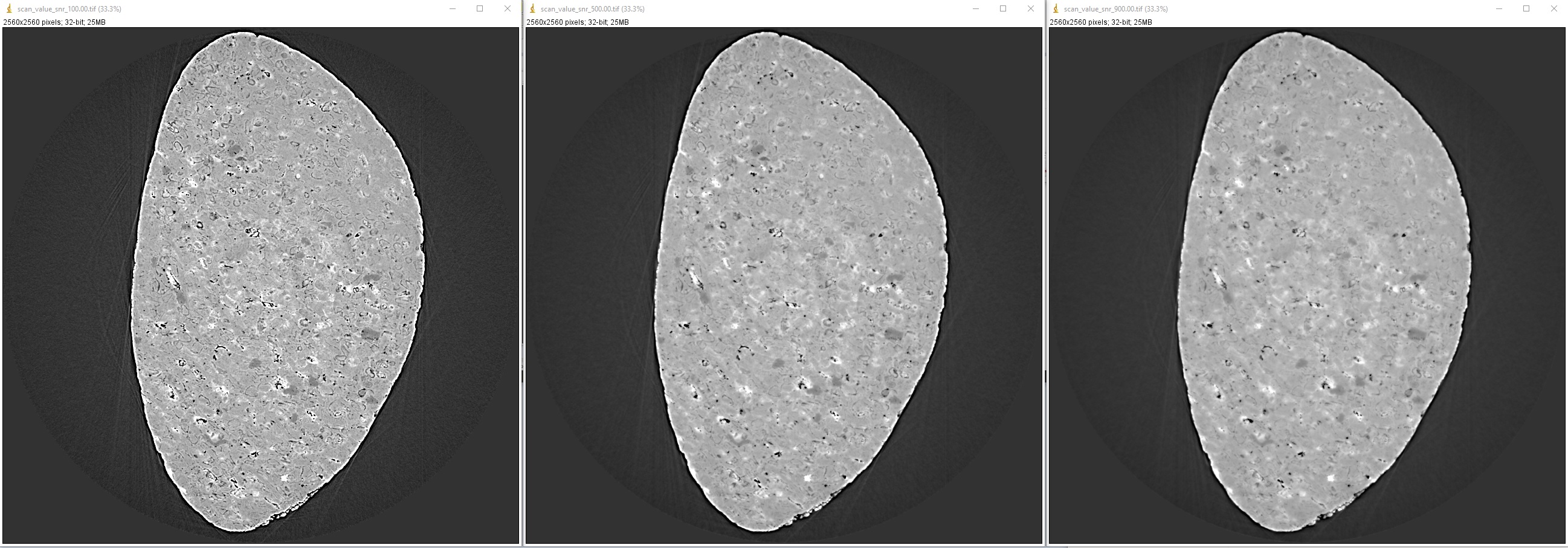
To perform scanning a parameter of a ring removal method
# To create new output-folder for each time of running the script.
output_base0 = "E:/tmp/scan_parameters/"
folder_name = losa.make_folder_name(output_base0, name_prefix="Scan_ratio", zero_prefix=3)
output_base = output_base0 + "/" + folder_name + "/"

for value in np.linspace(1.1, 3.0, 20):
    sinogram1 = remo.remove_all_stripe(sinogram, snr=value, la_size=51, sm_size=21)
    name = "snr_{0:2.2f}".format(value)
    rec_img = rec.fbp_reconstruction(sinogram1, center)
    losa.save_image(output_base + "/scan_value_" + name + ".tif", rec_img)
or a contrast-enhancement method
for ratio in np.arange(100, 1600, 400):
    sinogram1 = filt.fresnel_filter(sinogram, ratio, dim=1)
    name = "snr_{0:4.2f}".format(ratio)
    rec_img = rec.fbp_reconstruction(sinogram1, center)
    losa.save_image(output_base + "/scan_value_" + name + ".tif", rec_img)
4.5.5. Choosing a reconstruction method
The quality of reconstructed data in synchrotron-based X-ray microtomography depends heavily on the preprocessing methods applied. If the number of acquired projections is standard and the data are properly cleaned, the choice of reconstruction method will have less impact on the quality of the final results. Therefore, users can choose a reconstruction method based on the availability of computing resources.
output_base = "E:/tmp/compare_reconstruction_methods/"

# Using the direct Fourier inversion method (CPU)
t0 = timeit.default_timer()
rec_img = rec.dfi_reconstruction(sinogram, center)
print("Reconstructed image size: {}".format(rec_img.shape))
losa.save_image(output_base + "/DFI_method_cpu.tif", rec_img)
t1 = timeit.default_timer()
print("Using the DFI method (CPU). Time: {}".format(t1 - t0))

# Using the filtered back-projection method (CPU)
t0 = timeit.default_timer()
rec_img = rec.fbp_reconstruction(sinogram, center, gpu=False)
losa.save_image(output_base + "/FBP_method_cpu.tif", rec_img)
t1 = timeit.default_timer()
print("Using the FBP method (CPU). Time: {}".format(t1 - t0))

# Using the filtered back-projection method (GPU)
t0 = timeit.default_timer()
rec_img = rec.fbp_reconstruction(sinogram, center, gpu=True)
losa.save_image(output_base + "/FBP_method_gpu.tif", rec_img)
t1 = timeit.default_timer()
print("Using the FBP method (GPU). Time: {}".format(t1 - t0))

# Using the gridrec method (CPU)
t0 = timeit.default_timer()
rec_img = rec.gridrec_reconstruction(sinogram, center, ncore=1)
losa.save_image(output_base + "/gridrec_method_cpu.tif", rec_img)
t1 = timeit.default_timer()
print("Using the gridrec method (CPU). Time: {}".format(t1 - t0))
>>> Reconstructed image size: (2560, 2560) Using the DFI method (CPU). Time: 12.7383788 Using the FBP method (CPU). Time: 5.827241100000002 Using the FBP method (GPU). Time: 3.001648600000003 Using the gridrec method (CPU). Time: 1.7366413999999963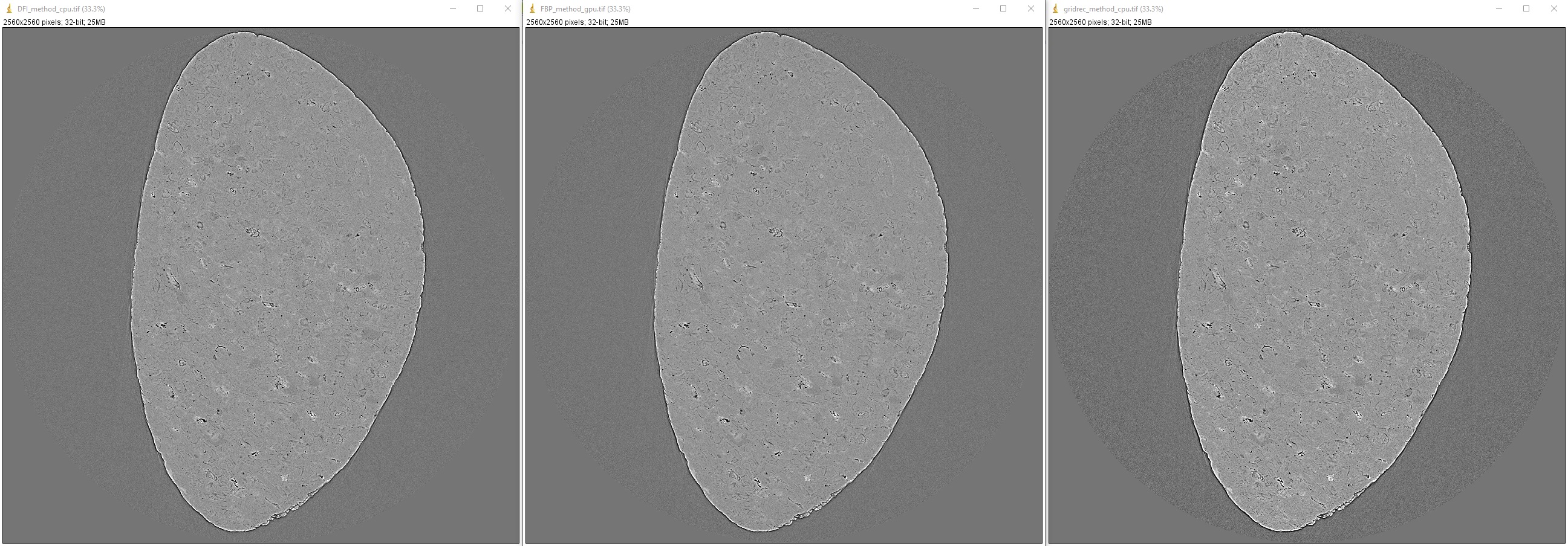
When dealing with undersampled sinogram, iterative reconstruction methods like SIRT (Simultaneous iterative reconstruction technique) can be advantageous over Fourier-based methods. However, iterative methods are computationally expensive. A workaround is to improve the Fourier-based methods by applying denoising and upsampling methods (Algotom >=1.3) to the sinogram.
output_base = "E:/tmp/improve_fft_method/"

print("Sinogram size {}".format(sinogram.shape))
# Using FBP method
rec_img1 = rec.fbp_reconstruction(sinogram, center, filter_name="hann")
losa.save_image(output_base + "/fbp_recon.tif", rec_img1)

# Using SIRT method with 150 number of iterations
rec_img2 = rec.astra_reconstruction(sinogram, center, method="SIRT_CUDA", num_iter=150)
losa.save_image(output_base + "/sirt_recon.tif", rec_img2)

# Denosing + upsampling sinogram + FBP reconstruction
sinogram = filt.fresnel_filter(sinogram, 100)
sinogram = corr.upsample_sinogram(sinogram, 2, center)
print("Upsampled sinogram size {}".format(sinogram.shape))
rec_img3 = rec.fbp_reconstruction(sinogram, center, filter_name="hann")
losa.save_image(output_base + "/fbp_denoising_upsampling.tif", rec_img3)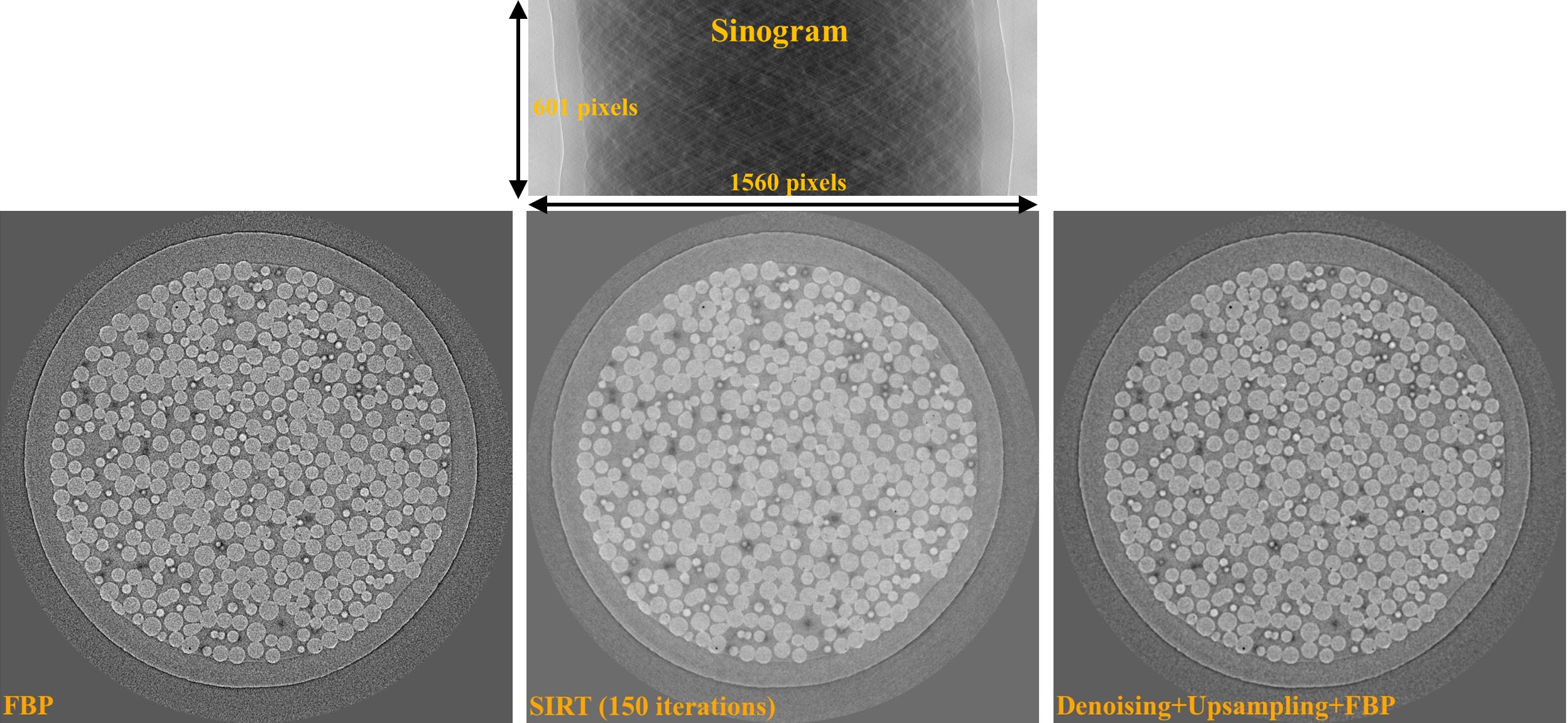
4.5.6. Performing full reconstruction
After completing all the steps for selecting parameters and testing methods, we can proceed with the full reconstruction process. The main difference compared to the previous steps is that sinograms are processed in chunks, which reduces I/O overhead and utilizes parallel processing. The following codes are available here for both tif and hdf input formats, but we can break down the workflow and provide detailed explanations:
Import the necessary modules from Algotom, specify the input and output paths, and add options to make it easier to modify the workflow later on.
import numpy as np
import timeit
import algotom.io.loadersaver as losa
import algotom.prep.correction as corr
import algotom.prep.calculation as calc
import algotom.rec.reconstruction as rec
import algotom.prep.removal as remo
import algotom.prep.filtering as filt
import algotom.util.utility as util

# Input file
file_path = "E:/Tomo_data/scan_68067.hdf"

# Specify output path, create new folder each time of running to avoid overwriting data.
output_base0 = "E:/full_reconstruction/"
folder_name = losa.make_folder_name(output_base0, name_prefix="recon", zero_prefix=3)
output_base = output_base0 + "/" + folder_name + "/"

# Optional parameters
start_slice = 10
stop_slice = -1
chunk = 100  # Number of slices to be reconstructed in one go. Adjust to suit RAM or GPU memory.
ncore = 16  # Number of cpu-core for parallel processing. Set to None for autoselecting.
output_format = "tif"  # "tif" or "hdf".
preprocessing = True  # Clean data before reconstruction.

# Give alias to a reconstruction method which is convenient for later change
# recon_method = rec.dfi_reconstruction
recon_method = rec.fbp_reconstruction
# recon_method = rec.gridrec_reconstruction # Fast cpu-method. Must install Tomopy.
# recon_method = rec.astra_reconstruction # To use iterative methods. Must install Astra.

# Provide metadata for loading hdf file, get data shape and rotation angles.
proj_path = "/entry/projections"
flat_path = "/entry/flats"
dark_path = "/entry/darks"
angle_path = "/entry/rotation_angle"
Load dark-field images, flat-field images, rotation angles; and calculate the center of rotation.
t_start = timeit.default_timer()
print("---------------------------------------------------------------")
print("-----------------------------Start-----------------------------\n")
print("1 -> Load dark-field and flat-field images, average each result")
# Load data, average flat and dark images, get data shape and rotation angles.
proj_obj = losa.load_hdf(file_path, proj_path)  # hdf object
(depth, height, width) = proj_obj.shape
flat_field = np.mean(np.asarray(losa.load_hdf(file_path, flat_path)), axis=0)
dark_field = np.mean(np.asarray(losa.load_hdf(file_path, dark_path)), axis=0)
angles = np.deg2rad(np.squeeze(np.asarray(losa.load_hdf(file_path, angle_path))))
(depth, height, width) = proj_obj.shape

print("2 -> Calculate the center-of-rotation")
# Extract sinogram at the middle for calculating the center of rotation
index = height // 2
sinogram = corr.flat_field_correction(proj_obj[:, index, :], flat_field[index, :],
                                      dark_field[index, :])
center = calc.find_center_vo(sinogram)
print("Center-of-rotation is {}".format(center))
Loop through the sinograms chunk-by-chunk, apply the selected pre-processing methods in parallel, and perform the reconstruction.
if (stop_slice == -1) or (stop_slice > height):
    stop_slice = height
total_slice = stop_slice - start_slice
if output_format == "hdf":
    # Note about the change of data-shape
    recon_hdf = losa.open_hdf_stream(output_base + "/recon_data.hdf",
                                     (total_slice, width, width),
                                     key_path='entry/data',
                                     data_type='float32', overwrite=True)
t_load = 0.0
t_prep = 0.0
t_rec = 0.0
t_save = 0.0
chunk = np.clip(chunk, 1, total_slice)
last_chunk = total_slice - chunk * (total_slice // chunk)

# Perform full reconstruction
for i in np.arange(start_slice, start_slice + total_slice - last_chunk, chunk):
    start_sino = i
    stop_sino = start_sino + chunk
    # Load data, perform flat-field correction
    t0 = timeit.default_timer()
    sinograms = corr.flat_field_correction(
        proj_obj[:, start_sino:stop_sino, :],
        flat_field[start_sino:stop_sino, :],
        dark_field[start_sino:stop_sino, :])
    t1 = timeit.default_timer()
    t_load = t_load + t1 - t0

    # Perform pre-processing
    if preprocessing:
        t0 = timeit.default_timer()
        # Algotom < 1.6
        # sinograms = util.apply_method_to_multiple_sinograms(sinograms,
        #                                                     "remove_zinger",
        #                                                     [0.08, 1],
        #                                                     ncore=ncore,
        #                                                     prefer="threads")
        # sinograms = util.apply_method_to_multiple_sinograms(sinograms,
        #                                                     "remove_all_stripe",
        #                                                     [3.0, 51, 21],
        #                                                     ncore=ncore,
        #                                                     prefer="threads")
        # sinograms = util.apply_method_to_multiple_sinograms(sinograms,
        #                                                     "fresnel_filter",
        #                                                     [200, 1],
        #                                                     ncore=ncore,
        #                                                     prefer="threads")
        # Algotom >= 1.6
        sinograms = util.parallel_process_slices(sinograms, remo.remove_zinger,
                                                 [0.08, 1], ncore=ncore,
                                                 prefer="threads")
        sinograms = util.parallel_process_slices(sinograms,
                                                 remo.remove_all_stripe,
                                                 [3.0, 51, 21], ncore=ncore,
                                                 prefer="threads")
        sinograms = util.parallel_process_slices(sinograms,
                                                 filt.fresnel_filter,
                                                 [200, 1], ncore=ncore,
                                                 prefer="threads")
        t1 = timeit.default_timer()
        t_prep = t_prep + t1 - t0

    # Perform reconstruction
    t0 = timeit.default_timer()
    recon_imgs = recon_method(sinograms, center, angles=angles, ncore=ncore)
    t1 = timeit.default_timer()
    t_rec = t_rec + t1 - t0

    # Save output
    t0 = timeit.default_timer()
    if output_format == "hdf":
        recon_hdf[start_sino - start_slice:stop_sino - start_slice] = np.moveaxis(recon_imgs, 1, 0)
    else:
        for j in range(start_sino, stop_sino):
            out_file = output_base + "/rec_" + ("0000" + str(j))[-5:] + ".tif"
            losa.save_image(out_file, recon_imgs[:, j - start_sino, :])
    t1 = timeit.default_timer()
    t_save = t_save + t1 - t0
    t_stop = timeit.default_timer()
    print("Done slice: {0} - {1} . Time {2}".format(start_sino, stop_sino,
                                                    t_stop - t_start))
if last_chunk != 0:
    start_sino = start_slice + total_slice - last_chunk
    stop_sino = start_sino + last_chunk

    # Load data, perform flat-field correction
    t0 = timeit.default_timer()
    sinograms = corr.flat_field_correction(
        proj_obj[:, start_sino:stop_sino, :],
        flat_field[start_sino:stop_sino, :],
        dark_field[start_sino:stop_sino, :])
    t1 = timeit.default_timer()
    t_load = t_load + t1 - t0

    # Perform pre-processing
    if preprocessing:
        t0 = timeit.default_timer()
        # Algotom < 1.6
        # sinograms = util.apply_method_to_multiple_sinograms(sinograms,
        #                                                     "remove_zinger",
        #                                                     [0.08, 1],
        #                                                     ncore=ncore,
        #                                                     prefer="threads")
        # sinograms = util.apply_method_to_multiple_sinograms(sinograms,
        #                                                     "remove_all_stripe",
        #                                                     [3.0, 51, 21],
        #                                                     ncore=ncore,
        #                                                     prefer="threads")
        # sinograms = util.apply_method_to_multiple_sinograms(sinograms,
        #                                                     "fresnel_filter",
        #                                                     [200, 1],
        #                                                     ncore=ncore,
        #                                                     prefer="threads")
        # Algotom >= 1.6
        sinograms = util.parallel_process_slices(sinograms, remo.remove_zinger,
                                                 [0.08, 1], ncore=ncore,
                                                 prefer="threads")
        sinograms = util.parallel_process_slices(sinograms,
                                                 remo.remove_all_stripe,
                                                 [3.0, 51, 21], ncore=ncore,
                                                 prefer="threads")
        sinograms = util.parallel_process_slices(sinograms,
                                                 filt.fresnel_filter,
                                                 [200, 1], ncore=ncore,
                                                 prefer="threads")
        t1 = timeit.default_timer()
        t_prep = t_prep + t1 - t0

    # Perform reconstruction
    t0 = timeit.default_timer()
    recon_imgs = recon_method(sinograms, center, angles=angles, ncore=ncore)
    t1 = timeit.default_timer()
    t_rec = t_rec + t1 - t0

    # Save output
    t0 = timeit.default_timer()
    if output_format == "hdf":
        recon_hdf[start_sino - start_slice:stop_sino - start_slice] = np.moveaxis(recon_imgs, 1, 0)
    else:
        for j in range(start_sino, stop_sino):
            out_file = output_base + "/rec_" + ("0000" + str(j))[-5:] + ".tif"
            losa.save_image(out_file, recon_imgs[:, j - start_sino, :])
    t1 = timeit.default_timer()
    t_save = t_save + t1 - t0
    t_stop = timeit.default_timer()
    print("Done slice: {0} - {1} . Time {2}".format(start_sino, stop_sino,
                                                    t_stop - t_start))
print("---------------------------------------------------------------")
print("-----------------------------Done-----------------------------")
print("Loading data cost: {0:0.2f}s".format(t_load))
print("Preprocessing cost: {0:0.2f}s".format(t_prep))
print("Reconstruction cost: {0:0.2f}s".format(t_rec))
print("Saving output cost: {0:0.2f}s".format(t_save))
print("Total time cost : {0:0.2f}s".format(t_stop - t_start))
>>>
---------------------------------------------------------------
-----------------------------Start-----------------------------

1 -> Load dark-field and flat-field images, average each result
2 -> Calculate the center-of-rotation
Center-of-rotation is 1272.75
Done slice: 10 - 110 . Time 189.6021034
Done slice: 110 - 210 . Time 366.9538149
Done slice: 210 - 310 . Time 579.1721645
Done slice: 310 - 410 . Time 783.6394176
Done slice: 410 - 510 . Time 1001.0833168
Done slice: 510 - 610 . Time 1206.3565348
Done slice: 610 - 710 . Time 1415.9822423
Done slice: 710 - 810 . Time 1630.9875868
Done slice: 810 - 910 . Time 1844.1762275
Done slice: 910 - 1010 . Time 2052.5243417
Done slice: 1010 - 1110 . Time 2266.1704849000002
Done slice: 1110 - 1210 . Time 2485.4279775
Done slice: 1210 - 1310 . Time 2695.1756578000004
Done slice: 1310 - 1410 . Time 2902.663489
Done slice: 1410 - 1510 . Time 3122.5606983000002
Done slice: 1510 - 1610 . Time 3333.1580989000004
Done slice: 1610 - 1710 . Time 3545.0758953000004
Done slice: 1710 - 1810 . Time 3758.1900975000003
Done slice: 1810 - 1910 . Time 3974.6899012000003
Done slice: 1910 - 2010 . Time 4181.2648382
Done slice: 2010 - 2110 . Time 4389.6914713999995
Done slice: 2110 - 2160 . Time 4511.7352912
---------------------------------------------------------------
-----------------------------Done-----------------------------
Loading data cost: 675.88s
Preprocessing cost: 3213.10s
Reconstruction cost: 337.11s
Saving output cost: 276.67s
Total time cost : 4511.74s
As shown in the time cost list above, the most time-consuming step is pre-processing, specifically the remove_all_stripe method, which relies on the median filter. Although other options for faster ring removal methods are available, parameter tweaking may be required for individual slices or datasets within the same experiment, which is impractical. The advantage of the remove_all_stripe method is that the same set of parameters can be applied to the entire volume and different datasets.
4.5.7. Automating the workflow
In practice, we often need to reconstruct not just one but hundreds or even thousands of datasets per synchrotron beamtime. In these cases, manually processing each dataset would be time-consuming and impractical. Instead, we can leverage the power of Python to automate the workflow. The idea is to create a Python script that can iterate through a list of datasets and pass the path of each dataset to the full reconstruction script for processing, either one-by-one on a local workstation or in parallel on a cluster.
We need to modify the full-reconstruction script to accept the file path as a command-line argument. This will allow us to pass the file path to the script dynamically from our automation script. There are several ways of doing this:
Using the sys module:
Modify the top of the full reconstruction script:
#  Script to perform full reconstruction, named full_reconstruction.py
import sys
import time
import timeit
import numpy as np
import algotom.io.loadersaver as losa
import algotom.util.utility as util
import algotom.prep.correction as corr
import algotom.prep.calculation as calc
import algotom.prep.removal as remo
import algotom.prep.filtering as filt
import algotom.rec.reconstruction as rec


file_path = sys.argv[1]  #  sys.argv[0] is the name of this script.
output_base = sys.argv[2]
# To pass arguments to this script, run:
# python full_reconstruction.py arg1 arg2

print("Load file: {}".format(file_path))
#  Script body ...
Then use the automation script as follows:
#  Script to call the full reconstruction script
import glob
import subprocess

python_interpreter = "C:/Users/nvo/Miniconda3/envs/algotom/python"
python_script = "full_reconstruction.py" #  At the same location of this script. Otherwise,
                                         #  providing the full path to full_reconstruction.py

input_folder = "E:/datasets/"
output_base = "E:/full_reconstruction/"
# Get a list of hdf files in the input folder.
list_file = glob.glob(input_folder + "/*hdf")

for file in list_file:
    script = python_interpreter + " " + python_script + " " + file.replace("\\", "/") + " " + output_base
    subprocess.call(script, shell=True)
Using the argparse module:
Modify the full reconstruction script as below:
#  Script to perform full reconstruction, named full_reconstruction.py
import argparse
import time
import timeit
import numpy as np
import algotom.io.loadersaver as losa
import algotom.util.utility as util
import algotom.prep.correction as corr
import algotom.prep.calculation as calc
import algotom.prep.removal as remo
import algotom.prep.filtering as filt
import algotom.rec.reconstruction as rec


parser = argparse.ArgumentParser(description="Perform full reconstruction")
parser.add_argument("-i", dest="file_path", help="Path to input file", type=str, required=True)
parser.add_argument("-o", dest="output", help="Output folder", type=str, required=True)
args = parser.parse_args()
# To pass arguments to this script, run:
# python full_reconstruction.py -i file_path -o output

file_path = args.file_path
output_base = args.output

print("Load file: {}".format(file_path))
#  Script body ...
Then just slightly modify the automation script:
#  Script to call the full reconstruction script
import glob
import subprocess

python_interpreter = "C:/Users/nvo/Miniconda3/envs/algotom/python"
python_script = "full_reconstruction.py" #  At the same location of this script. Otherwise,
                                         #  providing the full path to full_reconstruction.py

input_folder = "E:/datasets/"
output_base = "E:/full_reconstruction/"
# Get a list of hdf files in the input folder.
list_file = glob.glob(input_folder + "/*hdf")

for file in list_file:
    script = python_interpreter + " " + python_script + " -i " + file.replace("\\", "/") + " -o " + output_base
    subprocess.call(script, shell=True)
The instructions above are for running the reconstruction on a local machine (WinOS). However, if users have access to a cluster system (LinuxOS), they can take advantage of its resources to process multiple datasets in parallel using an embarrassingly parallel approach. The procedure of how to run reconstruction process on a cluster is as follows:
Install Python packages. Although a cluster may already have a standard Python environment with a set of pre-installed packages, it may not include the package users need. In this case, users can create their own Python environment. There are several ways to create a new Python environment, but one popular method is to use conda. Conda is a package management system that makes it easy to create, manage environments and packages. One of the advantages of conda is that it includes many popular Python packages, and it also includes pip, which allows users to install packages only available on PyPI.org. If conda is not installed on the cluster system, users can follow instructions here to install it, then installing Python packages as shown here.
Insert the full-path to the Python interpreter of the created environment at the top of python scripts:
#!/path/to/python/environment/bin/python

#  Script to perform full reconstruction, named full_reconstruction.py
import sys
# ...
then making the file executable by run the following command in a Linux terminal:
chmod +x <filename>Write a bash script to submit jobs to the cluster scheduler. The bash script can be embed inside a Python script to make it easy to customize the workflow. The following example demonstrates how to do that for a SLURM cluster scheduler (for Univa Grid Engine scheduler, refer the example here):
#!/path/to/python/environment/bin/python

import os
import glob
import subprocess

python_script = "full_reconstruction.py"
use_gpu = True
input_folder = "/facility/beamline/data/year/proposals/visit/raw_data/"
# Get a list of nxs files in the input folder.
list_file = glob.glob(input_folder + "/*nxs")
# Specify where to save the processed data
output_base = "/facility/beamline/data/year/proposals/visit/processing/reconstruction"
# Specify the folder for cluster output-file and error-file.
cluster_dir = "/facility/beamline/data/year/proposals/visit/processing/cluster_output/"

# Define a method to create a folder for saving output message from the cluster.
def make_folder(folder_path):
    file_base = os.path.dirname(folder_path)
    if not os.path.exists(file_base):
        try:
            os.makedirs(file_base)
        except FileExistsError:
            pass
        except OSError:
            raise ValueError("Can't create the folder: {}".format(file_base))

sbatch_script_cpu = """#!/bin/bash

#SBATCH --job-name=demo_workflow
#SBATCH --ntasks 1
#SBATCH --cpus-per-task 16
#SBATCH --nodes=1
#SBATCH --mem=16G
#SBATCH --qos=normal
#SBATCH --time=60:00

srun -o {0}/output_%j.txt -e {0}/error_%j.txt ./{1} {2} {3}
"""

sbatch_script_gpu = """#!/bin/bash

#SBATCH --job-name=demo_workflow
#SBATCH --ntasks 1
#SBATCH --cpus-per-task 16
#SBATCH --nodes=1
#SBATCH --mem=16G
#SBATCH --gres=gpu:1
#SBATCH --qos=normal
#SBATCH --time=60:00

srun -o {0}/output_%j.txt -e {0}/error_%j.txt ./{1} {2} {3}
"""

for file_path in list_file:
    file_name = os.path.basename(file_path)
    name = file_name.replace(".nxs", "")
    output_folder = output_base + "/" + file_name + "/"
    print("Submit to process the raw-data file : {}...".format(file_name))
    cluster_output = cluster_dir + "/" + name + "/"
    make_folder(cluster_output)
    if use_gpu:
        sbatch_script = sbatch_script_gpu.format(cluster_output, python_script,
                                                 file_path, output_folder)
    else:
        sbatch_script = sbatch_script_cpu.format(cluster_output, python_script,
                                                 file_path, output_folder)
    # Call sbatch and pass the sbatch script contents as input
    process = subprocess.Popen(['sbatch'], stdin=subprocess.PIPE, stdout=subprocess.PIPE, stderr=subprocess.PIPE)
    stdout, stderr = process.communicate(input=sbatch_script.encode())

    # Print the output and error messages
    print(stdout.decode())
    print(stderr.decode())
print("*********************************************")
print("             !!!!!! Done !!!!!!              ")
print("*********************************************")
To run the script, make it executable and log in to a submitting job node. Users can modify the workflow above by reconstructing multiple datasets at once, such as 10 datasets in one batch, and waiting for them to finish before submitting another batch. This approach ensures fair use of cluster resources among multiple users.
4.5.8. Downsampling, rescaling, and reslicing reconstructed volume
Reconstructed volume is in 32-bit tif or hdf format. In the above example, the size of the volume is 2150 x 2560 x 2560 pixels, which corresponds to ~50 GB of data. To enable post-analysis on software for volume visualization and analysis; e.g. Avizo, Amira, DragonFly, Drishti, Paraview, 3D Slicer, …; it is often necessary to apply data reduction techniques such as cropping, downsampling, or rescaling. Algotom provides convenient functions for these tasks, which can be applied to a folder of tif slices or a hdf/nxs file.
import timeit
import algotom.io.loadersaver as losa
import algotom.post.postprocessing as post

output_base = "E:/output/data_reduction/"

# Rescale the volume to 16-bit data including cropping.
# Input is tif, output is tif
tif_folder = "E:/full_reconstruction/recon_001"
output0 = output_base + "/rescaling/"
folder_name = losa.make_folder_name(output0)  # To avoid overwriting
output = output0 + "/" + folder_name + "/"
t_start = timeit.default_timer()
post.rescale_dataset(tif_folder, output, nbit=16, minmax=None, skip=None,
                     crop=(100, 100, 200, 200, 200, 200))

# # Input is hdf, output is tif
# file_path = "E:/full_reconstruction/recon_002/recon_data.hdf"
# key_path = "entry/data"
# post.rescale_dataset(file_path, output, key_path=key_path, nbit=16, minmax=None,
#                      skip=None, crop=(100, 100, 200, 200, 200, 200))
t_stop = timeit.default_timer()
print("Done rescaling! Time cost {}".format(t_stop - t_start))


# Downsample the volume by 2 x 2 x 2 with cropping and rescaling to 8-bit.
output0 = output_base + "/downsampling/"
folder_name = losa.make_folder_name(output0)  # To avoid overwriting
output = output0 + "/" + folder_name + "/"
t_start = timeit.default_timer()
post.downsample_dataset(tif_folder, output, (2, 2, 2), method='mean',
                        rescaling=True, nbit=8, minmax=None, skip=None,
                        crop=(100, 100, 200, 200, 200, 200))
t_stop = timeit.default_timer()
print("Done downsampling! Time cost {}".format(t_stop - t_start))
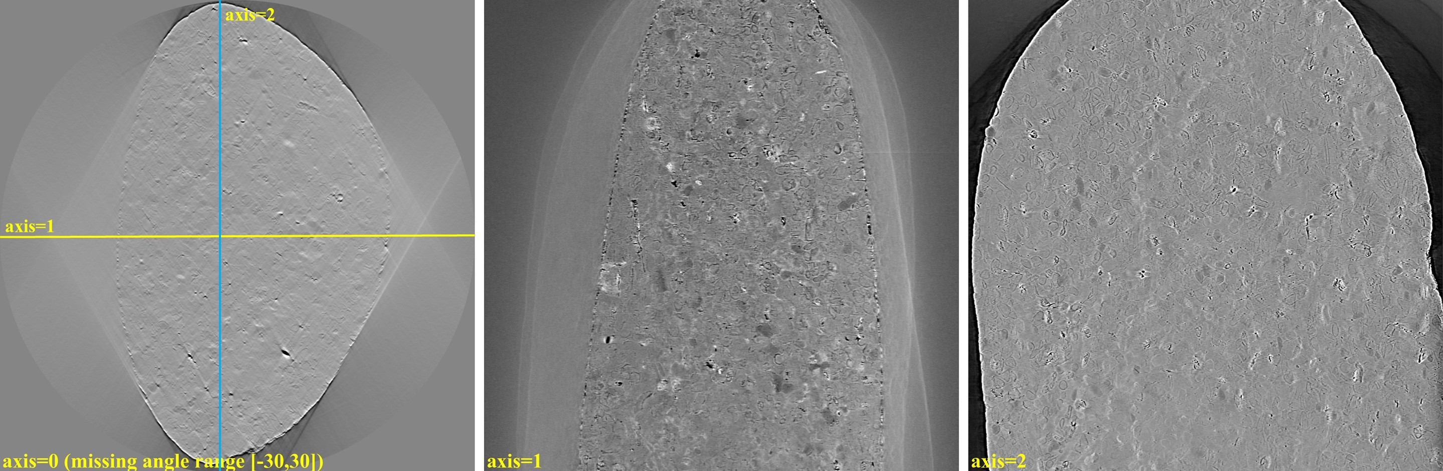
Reslicing the reconstructed volume is another important post-processing tool, especially for limited-angle tomography. While some software such as ImageJ or Avizo offer this function, they require loading the entire volume into memory, making it impossible to use on computers with limited RAM. Starting from version 1.3, Algotom provides a reslicing function that uses the hdf format as the back-end, eliminating the need for high memory usage. Additionally, options for cropping, rotating, and rescaling the volume are also included.
import timeit
import algotom.io.loadersaver as losa
import algotom.post.postprocessing as post

output_base = "E:/output/reslicing"

# Reslice the volume along axis 1, including rotating, cropping, and rescaling to 8-bit data.
# Input is tif, output is tif
tif_folder = "E:/full_reconstruction/recon_001"
folder_name = losa.make_folder_name(output_base)  # To avoid overwriting
output = output_base + "/" + folder_name + "/"
t_start = timeit.default_timer()

post.reslice_dataset(tif_folder, output, rescaling=True, rotate=10.0,
                     nbit=8, axis=1, crop=(100, 100, 200, 200, 200, 200),
                     chunk=60, show_progress=True, ncore=None)

# # Input is hdf, output is tif. It's possible to slice a hdf volume directly
# # along axis 2 but it will be extremely slow. Better use the Algotom function as below.
#
# file_path = "E:/full_reconstruction/recon_002/recon_data.hdf"
# key_path = "entry/data"
# post.reslice_dataset(file_path, output, key_path=key_path, rescaling=True,
#                      rotate=0.0, nbit=16, axis=2, crop=(100, 100, 200, 200, 200, 200),
#                      chunk=60, show_progress=True, ncore=None)

t_stop = timeit.default_timer()
print("Done reslicing! Time cost {}".format(t_stop - t_start))
As shown below, reslicing along the direction perpendicular to the missing wedge can produce high-quality images suitable for post-analysis.
4.5.9. Common mistakes and useful tips
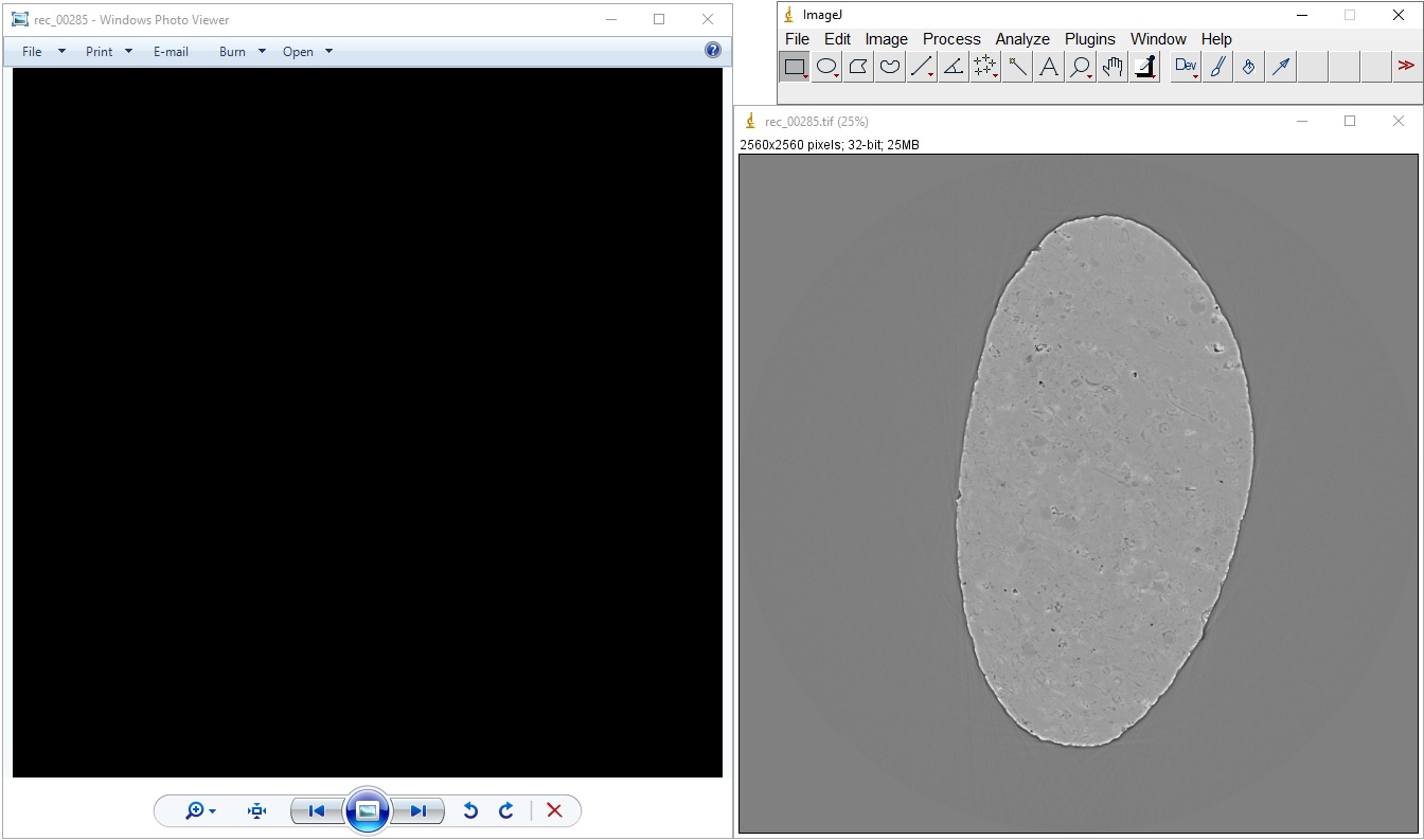
We may see black images when using viewer software that does not support 32-bit tif images. Users need to use ImageJ or Fiji to view 32-bit tif reconstructed slices or flat-field-corrected images.
Black reconstructed slice is returned due to the zero division problem. Reconstruction methods in Algotom apply the logarithm function to a sinogram by default, based on Beer-Lambert’s law. However, this can result in NaN values if there are zeros or negative values in the sinogram. Zeros or negative values may comes from phase-retrieved images or the flat-field correction process using projection images which may have the following:
Time stamp at one of the image corner.
Beam size is smaller than the field of view.
To address these issues, there are several ways:
Disable the logarithm function by setting apply_log to False in a reconstruction method if the input is a non-absorption-contrast image.
Crop the images to exclude problematic regions.
Not using dark-field image for low SNR data.
Replace zeros and negative values in the sinogram as below
import numpy as np
nmean = np.mean(sinogram)
sinogram[sinogram<=0.0] = nmean
Algotom provides a convenient method for flat-field correction; with the options to correct zero division, not use dark-field image, or include other preprocessing methods.
Users may apply methods on the wrong space or slice data along incorrect axis. As shown in Fig. 4.5.1, it is assumed that the sample is upright, and therefore the rotation axis is parallel to the columns of the projection image. In 3D data, axis 0 represents the projection space; axis 1 represents the sinogram space and the reconstruction space. It is important to ensure that methods are applied correctly to the appropriate space and that data is sliced along the correct axis. Sometimes the rotation axis of a tomography system may be parallel to the rows of the projection image. In such cases, users need to rotate the projection image or adjust the slicing direction to obtain the sinogram image.
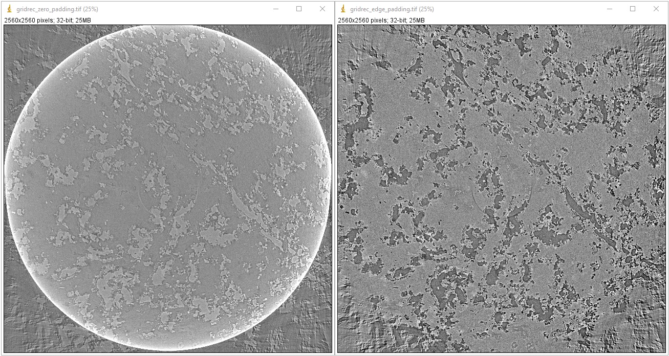
Cupping artifacts or outermost bright/dark ring artifacts can occur when padding is not used or wrong type of padding is used for Fourier-based reconstruction methods. This problem has a significant impact on post-analysis, particularly image segmentation, but very easy to fix simply by applying a proper padding such as ‘edge’, ‘reflect’, or ‘symmetric’. In Algotom, ‘edge’ padding is enabled by default for FFT-based methods, but in other software this function may not be enabled by default or zero-padding is used. The following image demonstrates the difference between using zero padding and edge padding for the gridrec method.
import tomopy
import algotom.io.loadersaver as losa
import algotom.prep.calculation as calc
import algotom.rec.reconstruction as rec

center = calc.find_center_vo(sinogram)
# Algotom wrapper provides edge-padding.
rec_img1 = rec.gridrec_reconstruction(sinogram, center, ratio=None)
# Tomopy applies zero-padding by default.
rec_img2 = tomopy.recon(np.expand_dims(sinogram, 1),
                        np.deg2rad(np.linspace(0, 180.0, sinogram.shape[0])),
                        center=center, algorithm="gridrec")

losa.save_image(output_base + "/gridrec_edge_padding.tif", rec_img1)
losa.save_image(output_base + "/gridrec_zero_padding.tif", rec_img2[0])
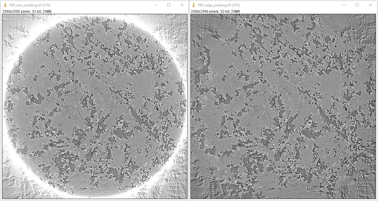
and demonstration for the FBP method:
import algotom.io.loadersaver as losa
import algotom.prep.calculation as calc
import algotom.rec.reconstruction as rec

center = calc.find_center_vo(sinogram)
# Using built-in FBP method in Algotom with edge padding.
rec_img1 = rec.fbp_reconstruction(sinogram, center, ratio=None)
# Using FBP through Astra Toolbox. Astra applies zero-padding behind the scene.
# The Algotom wrapper provides edge-padding in addition to Astra's zero-padding.
# However, the artifacts caused by the zero-padding can still persist, as it
# disrupts the intensities at the boundaries, which is problematic for
# Fourier-based methods.
rec_img2 = rec.astra_reconstruction(sinogram, center, ratio=None, method="FBP_CUDA", pad=0)

losa.save_image(output_base + "/FBP_edge_padding.tif", rec_img1)
losa.save_image(output_base + "/FBP_zero_padding.tif", rec_img2)
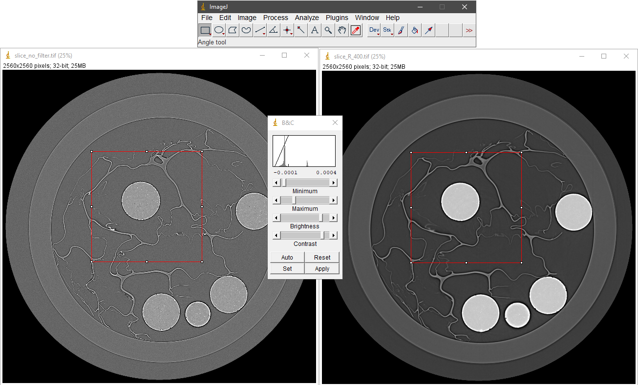
Users may not be aware of autoscaling implemented by image viewer software. Image viewers often apply autoscaling to account for differences in intensity range between different image types, such as 32-bit, 16-bit or 8-bit. However, this can lead to the displayed image having a contrast that does not accurately reflect the true contrast of the original image. The following shows examples of using the ImageJ software.
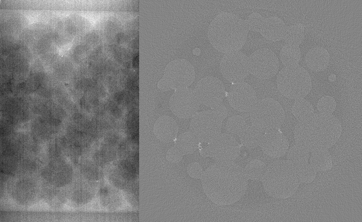
Commonly, users may select a ROI and adjust the contrast of the image by autoscaling as shown below. An autoscaling method works by normalizing the whole image based on the local minimum gray-scale and local maximum gray-scale of the ROI. As can be seen, the left-side image is more noisy and has a higher dynamic range of intensities (distance between the maximum intensity and minimum intensity) compared to the right-side image. When the auto-scaling is applied, the contrast of the right-side image is improved because it has lower dynamic range.
The following images shows the intensity profiles along the red lines in each image where the whole dynamic range of intensities are used to plot.
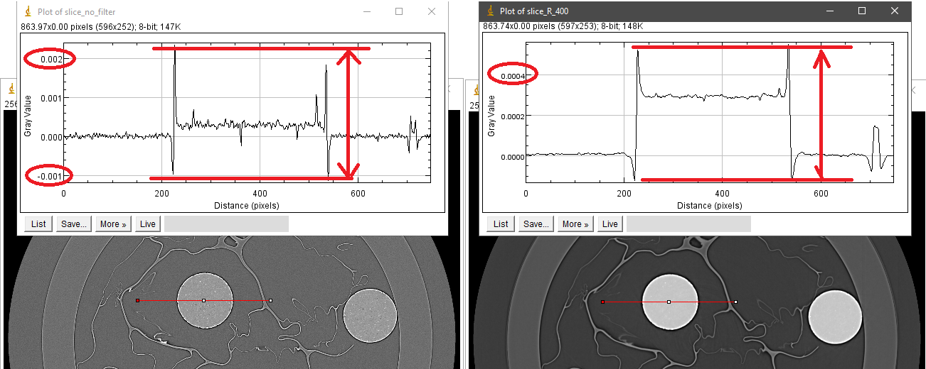
The following images show the intensity profiles along the red lines in each image where the dynamic range of intensities is set to be the same in both images. As can be seen, the gray-scale values of an Aluminum sphere are the same. Note that the intensities at the interfaces are strongly fluctuating due to the coherent effect of the X-ray source.
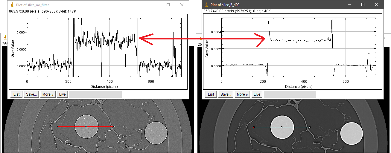
The above demonstration actually shows images reconstructed without and with Paganin filter (R=400), which was used to explain the common misconception that the resulting Paganin filter image is a phase-contrast image. From a mathematical point of view, Paganin’s formula is a low-pass filter in Fourier space, with R as a tuning parameter that controls the strength of this filter. As a low-pass filter, it reduces noise and the dynamic range of an image, which can help enhance the contrast between low-contrast features. However, this can sometimes be confused with the phase effect, leading to the common misconception that the resulting image is a phase-contrast image.
Overlapping parallelization should be avoided as it can degrade performance. Many functions in Algotom are set to use multi-core by default. If users would like to write a wrapper on top to perform parallel work, such as processing multiple datasets, making sure that the ncore option in Algotom API is set to 1.
There are different ways of applying pre-processing methods to multiple-sinograms as shown below.
Using with flat-field correction method:
import algotom.util.utility as util
import algotom.prep.correction as corr
import algotom.prep.removal as remo
import algotom.prep.filtering as filt

opt1 = {"method": "remove_zinger", "para1": 0.08, "para2": 1}
opt2 = {"method": "remove_all_stripe", "para1": 3.0, "para2": 51, "para3": 17}
opt3 = {"method": "fresnel_filter", "para1": 200, "para2": 1}
sinograms = corr.flat_field_correction(proj_obj[:, 20:40, :], flat_field[20:40, :], dark_field[20:40, :],
                                       option1=opt1, option2=opt2, option3=opt3)
Applying methods one-by-one:
sinograms = corr.flat_field_correction(proj_obj[:, 20:40, :], flat_field[20:40, :], dark_field[20:40, :])
sino_pro = []
for i in range(sinograms.shape[1]):
    sino_tmp = remo.remove_zinger(sinograms[:, i, :], 0.08, 1)
    sino_tmp = remo.remove_all_stripe(sino_tmp, 3.0, 51, 17)
    sino_tmp = filt.fresnel_filter(sino_tmp, 200, 1)
    sino_pro.append(sino_tmp)
# Convert results which is a Python list to a Numpy array and
# make sure axis 1 is corresponding to sinogram.
sinograms = np.moveaxis(np.asarray(sino_pro), 0, 1)
Applying methods in parallel manually:
import multiprocessing as mp
from joblib import Parallel, delayed

ncore = mp.cpu_count() - 1
sinograms = corr.flat_field_correction(proj_obj[:, 20:40, :], flat_field[20:40, :], dark_field[20:40, :])
num_sino = sinograms.shape[1]

output_tmp = Parallel(n_jobs=ncore, prefer="threads")(delayed(
    remo.remove_zinger)(sinograms[:, j, :], 0.08, 1) for j in range(num_sino))
sinograms = np.moveaxis(np.asarray(output_tmp), 0, 1)

output_tmp = Parallel(n_jobs=ncore, prefer="threads")(delayed(
    remo.remove_all_stripe)(sinograms[:, j, :], 3.0, 51, 21) for j in
                                                      range(num_sino))
sinograms = np.moveaxis(np.asarray(output_tmp), 0, 1)

output_tmp = Parallel(n_jobs=ncore, prefer="threads")(delayed(
    filt.fresnel_filter)(sinograms[:, j, :], 200, 1) for j in range(num_sino))
sinograms = np.moveaxis(np.asarray(output_tmp), 0, 1)
Applying methods in parallel using Algotom API:
# Algotom < 1.6
# sinograms = corr.flat_field_correction(proj_obj[:, 20:40, :], flat_field[20:40, :], dark_field[20:40, :])
# sinograms = util.apply_method_to_multiple_sinograms(sinograms, "remove_zinger", [0.08, 1],
#                                                     ncore=None, prefer="threads")
# sinograms = util.apply_method_to_multiple_sinograms(sinograms, "remove_all_stripe", [3.0, 51, 17],
                                                    ncore=None, prefer="threads")
# sinograms = util.apply_method_to_multiple_sinograms(sinograms, "fresnel_filter", [200, 1],
                                                    ncore=None, prefer="threads")
# Algotom >= 1.6
sinograms = util.parallel_process_slices(sinograms, remo.remove_zinger,
                                         [0.08, 1], ncore=None,
                                         prefer="threads")
sinograms = util.parallel_process_slices(sinograms, remo.remove_all_stripe,
                                         [3.0, 51, 17], ncore=None,
                                         prefer="threads")
sinograms = util.parallel_process_slices(sinograms, filt.fresnel_filter,
                                         [200, 1], ncore=None,
                                         prefer="threads")
Starting from version 1.3, Algotom’s reconstruction methods support batch processing of multiple sinograms at once. It is important to note that the axis of the reconstructed slices is 1, which is similar to the axis used for extracting sinograms.
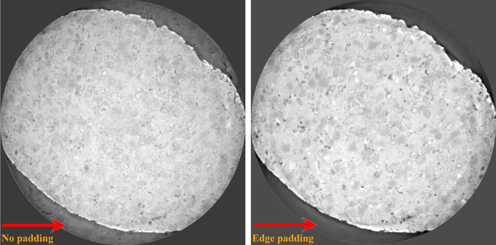
Padding must be used for any Fourier-based image processing method, not just reconstruction as demonstrated in tip 5, to reduce/remove side-effect artifacts. Without padding, well-used Fourier-based filters, such as Paganin filter or Fresnel filter, applied on projection images can produce barrel-shaped intensity profiles in reconstructed images
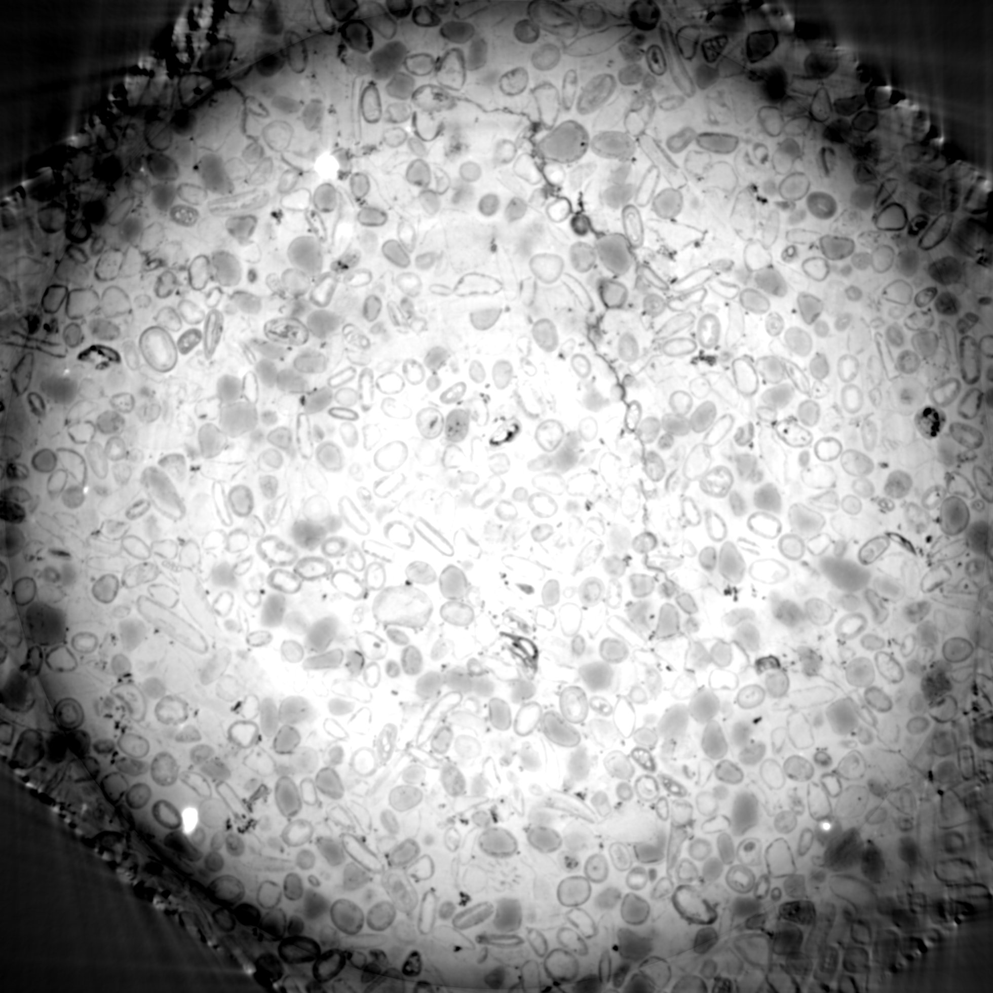
or ghost features in the top and bottom slices caused by cross-shaped artifacts in the frequency domain due to spectral leakage.
In some cases, a tomography system may not be well-aligned, resulting in a rotation axis that is not perpendicular to the rows of projection images. The angle of misalignment can be very small and difficult to detect or calculate using projection images alone. A more accurate method involves extracting sinograms at the top, middle, and bottom of the tomographic data (or more, to improve the fitting result later), calculating the center of rotation, and then applying a linear fit to the results to obtain the tilt angle of the rotation axis.
import numpy as np
import algotom.io.loadersaver as losa
import algotom.prep.correction as corr
import algotom.prep.calculation as calc
import algotom.rec.reconstruction as rec

file_path = "E:/Tomo_data/scan_68067.hdf"
output_base = "E:/output/tilted_projection/"
proj_path = "entry/projections"  # Refer section 1.2.1 to know how to get
                                 # path to a dataset in a hdf file.
flat_path = "entry/flats"
dark_path = "entry/darks"

# Load data, average flat and dark images
proj_obj = losa.load_hdf(file_path, proj_path)  # hdf object
(depth, height, width) = proj_obj.shape
flat_field = np.mean(np.asarray(losa.load_hdf(file_path, flat_path)), axis=0)
dark_field = np.mean(np.asarray(losa.load_hdf(file_path, dark_path)), axis=0)

# Find center at different height for calculating the tilt angle
slice_and_center = []
for i in range(10, height-10, height // 2 - 11):
    print("Find center at slice {}".format(i))
    sinogram = corr.flat_field_correction(proj_obj[:, i,:], flat_field[i], dark_field[i])
    center = calc.find_center_vo(sinogram)
    print("Center is {}".format(center))
    slice_and_center.append([i, center])
slice_and_center = np.asarray(slice_and_center)

# Find the tilt angle using linear fit.
# Note that the sign of the tilt angle need to be changed if the projection
# images are flipped left-right or up-down by some detectors.
tilt_angle = -np.rad2deg(np.arctan(
    np.polyfit(slice_and_center[:, 0], slice_and_center[:, 1], 1)[0]))
print("Tilt angle: {} (degree)".format(np.deg2rad(tilt_angle)))

# Given tilted angle we can extract a single sinogram for reconstruction:
idx = height // 2
sino_tilted = corr.generate_tilted_sinogram(proj_obj, idx, tilt_angle)
flat_line = corr.generate_tilted_profile_line(flat_field, idx, tilt_angle)
dark_line = corr.generate_tilted_profile_line(dark_field, idx, tilt_angle)
sino_tilted = corr.flat_field_correction(sino_tilted, flat_line, dark_line)
center = calc.find_center_vo(sino_tilted)
rec_img = rec.fbp_reconstruction(sino_tilted, center)
losa.save_image(output_base + "/recon.tif", rec_img)
# or for a chunk of sinogram:
start_idx = 20
stop_idx = 40
sinos_tilted = corr.generate_tilted_sinogram_chunk(proj_obj, start_idx, stop_idx, tilt_angle)
flats_tilted = corr.generate_tilted_profile_chunk(flat_field, start_idx, stop_idx, tilt_angle)
darks_tilted = corr.generate_tilted_profile_chunk(dark_field, start_idx, stop_idx, tilt_angle)
sinos_tilted = corr.flat_field_correction(sinos_tilted, flats_tilted, darks_tilted)
center = calc.find_center_vo(sinos_tilted[:, start_idx, :])
recs_img = rec.fbp_reconstruction(sinos_tilted, center)
for i in range(start_idx, stop_idx):
    name = ("0000" + str(i))[-5:]
    losa.save_image(output_base + "/recon/recon_" + name + ".tif", recs_img[:, i-start_idx, :])
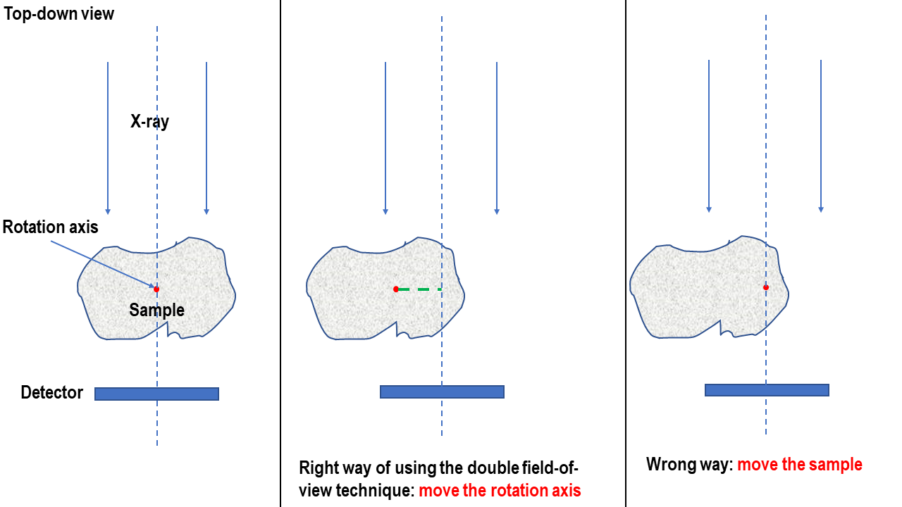
For increasing the field of view of the reconstructed image, the technique of 360-degree scan with offset rotation axis, also known as half-acquisition (though this can be a confusing name), is commonly used. However, it is important to note that the rotation axis should be shifted to the side of the field of view, not the sample itself. From the projection image, it can be confusing as both shifts give the same results.
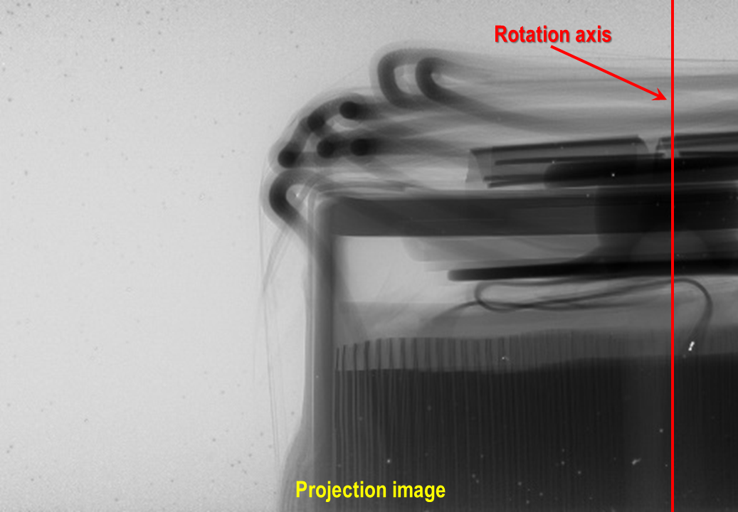
but it’s much easier to understand using the sketch below
4.5.10. Data analysis
After cleaning and reconstructing all slices, the next step is to analyze the data to answer scientific questions. There are a variety of tools and software available to users. For beginners, the following resources may be helpful:
For learning about the quantitative information that X-ray tomography can provide, a good starting point is the paper “Quantitative X-ray tomography” by E. Maire and P.J. Withers. This resource can provide a comprehensive overview of the field and help you understand the potential applications and benefits of this technique.
Tutorials on YouTube are one of the most effective ways to learn quickly:
Microscopy Australia channel: example talk.
Cscsch channel: example talk.
Channel of Dr. Sreenivas Bhattiprolu: tutorial playlists.